Page 44 - Introduction to Statistical Pattern Recognition

26 Introduction to Statistical Pattern Recognition

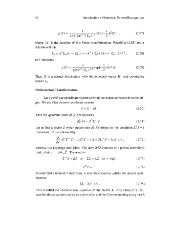
(2.67)

where IA I is the Jacobian of this linear transformation. Recalling (2.63) and a
determinant rule
C,=A~C~A+ I~~I=IA~II~,IIAI=IC~IIAI~, (2.68)
p (Y) becomes

(2.69)

Thus, Y is a normal distribution with the expected vector MY and covariance
matrix Xy.

Orthonormal Transformation

Let us shift our coordinate system to bring the expected vector M to the ori-
gin. We use Zfor the new coordinate system.
Z=X-M. (2.70)

Then the quadratic form of (2.22) becomes
&Z) = ZTC-IZ . (2.71)
Let us find a vector Z which maximizes d$(Z) subject to the condition ZTZ = 1
(constant). This is obtained by
a
-lzTC-lZ - p(Z7Z - 1)) = 2x-Iz - 2p.z = 0, (2.72)
az
where p is a Lagrange multiplier. The term a/aZ consists of n partial derivatives
[a/az a/az2 . . . &az,,lT. The result is
c-Iz=pz 01‘ zz =hZ (h = I/p), (2.73)

ZTZ= 1. (2.74)
In order that a nonnull Z may exist, h must be chosen to satisfy the determinant
equation
IC-hll =o. (2.75)

This is called the char-ucter-istic equatiori of the matrix Z. Any value of h that
satisfies this equation is called an eigenvalire, and the Z corresponding to a given h