Page 64 - Introduction to Statistical Pattern Recognition

46 Introduction to Statistical Pattern Recognition

otherwise, we use m =2.56, which gives the Bayes error of 10%. Also, unless
specified otherwise, we assume n = 8. Even when n changes, the Bayes error stays
the same for a fixed m.

Data 1-41:
m1 = . . . =m8 =O,

h, = . . . =A8 =4

In this data, the two expected vectors are the same, but the covariance
matrices are different. The Bayes error varies depending on the value of the hi’s as
well as n, and becomes about 9% for hl = . . . = h8 = 4. Again, unless specified
otherwise, we use n = 8 for this data.

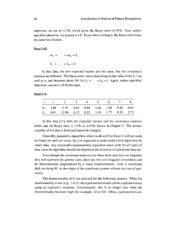
Data I-A:

I 1 2 3 4 5 6 7 8
mi 3.86 3.10 0.84 0.84 1.64 1.08 0.26 0.01
hi 8.41 12.06 0.12 0.22 1.49 1.77 0.35 2.73

In this data [ 1 11, both the expected vectors and the covariance matrices
differ, and the Bayes error is 1.9% as will be shown in Chapter 3. The dimen-
sionality of this data is fixed and cannot be changed.
Generally, parametric algorithms which work well for Data /-I will not work
for Data 1-41, and vice versa. So, it is important to understand which algorithms fit
which data. Any reasonable nonparametric algorithm must work for all types of
data, since the algorithm should not depend on the structure of a particular data set.

Even though the covariance matrices for these three data sets are diagonal,
they still represent the general case, since any two non-diagonal covariances can
be simultaneously diagonalized by a linear transformation. Also, a coordinate
shift can bring MI to the origin of the coordinate system without any loss of gen-
erality.
The dimensionality of 8 was selected for the following reasons. When the
dimensionality is low (e.g., 1 or 2), all experimental results can be explained easily
using an engineer’s intuition. Unfortunately, this is no longer true when the
dimensionality becomes high (for example, 32 or 64). Often, experimental con-