Page 70 - Introduction to Statistical Pattern Recognition

52 Introduction to Statistical Pattern Recognition

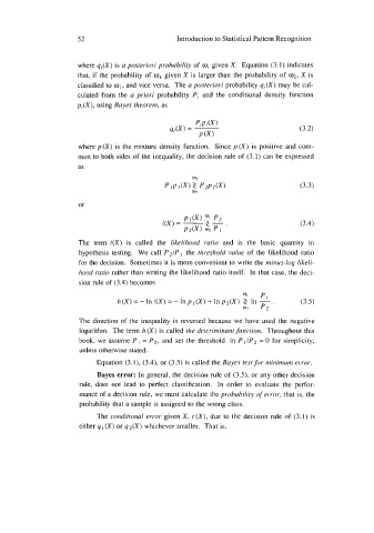
where qi(X) is a posteriori probability of 0; given X. Equation (3.1) indicates
that, if the probability of o1 given X is larger than the probability of 02, X is
classified to o1 , and vice versa. The a posteriori probability q;(X) may be cal-
culated from the a priori probability Pi and the conditional density function
pi(X), using Bayes theorem, as

(3.2)

where p (X) is the mixture density function. Since p (X) is positive and com-
mon to both sides of the inequality, the decision rule of (3.1) can be expressed
as

(3.3)

or

(3.4)

The term [(X) is called the likelihood ratio and is the basic quantity in
hypothesis testing. We call P21P the threshold value of the likelihood ratio
for the decision. Sometimes it is more convenient to write the minus-log likeli-
hood ratio rather than writing the likelihood ratio itself. In that case, the deci-
sion rule of (3.4) becomes
P,
h(X)=-lnt(X)=-InpI(X)+lnp2(X) 3 In -. (3.5)
02 p2
The direction of the inequality is reversed because we have used the negative
logarithm. The term h (X) is called the discriminant function. Throughout this
book, we assume P I = P 2, and set the threshold In P IIP = 0 for simplicity,
unless otherwise stated.
Equation (3.1), (3.4), or (3.5) is called the Bayes test for minimum error.
Bayes error: In general, the decision rule of (3.3, or any other decision
rule, does not lead to perfect classification. In order to evaluate the perfor-
mance of a decision rule, we must calculate the probability of error, that is, the
probability that a sample is assigned to the wrong class.
The conditional error given X, r(X), due to the decision rule of (3.1) is
either 9 I (X) or q*(X) whichever smaller. That is,