Page 35 - Petroleum Production Engineering, A Computer-Assisted Approach

Guo, Boyun / Computer Assited Petroleum Production Engg 0750682701_chap02 Final Proof page 24 22.12.2006 7:08pm

2/24 PETROLEUM PRODUCTION ENGINEERING FUNDAMENTALS
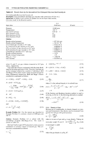
Table 2.3 Results Given by the Spreadsheet Carr-Kobayashi-Burrows-GasViscosity.xls
Carr-Kobayashi-Burrows-GasViscosity.xls
Description: This spreadsheet calculates gas viscosity with correlation of Carr et al.
Instruction: (1) Select a unit system; (2) update data in the Input data section;
(3) review result in the Solution section.
U.S.
Input data Field units SI units
Pressure: 10,000 psia
Temperature: 180 8F
Gas-specific gravity: 0.65 air ¼ 1
Mole fraction of N 2 : 0.1
Mole fraction of CO 2 : 0.08
Mole fraction of H 2 S: 0.02
Solution
Pseudo-critical pressure ¼ 697.164 psia
Pseudo-critical temperature ¼ 345.357 8R
Uncorrected gas viscosity at 14.7 psia ¼ 0.012174 cp
N 2 correction for gas viscosity at 14.7 psia ¼ 0.000800 cp
CO 2 correction for gas viscosity at 14.7 psia ¼ 0.000363 cp
H 2 S correction for gas viscosity at 14.7 psia ¼ 0.000043 cp
Corrected gas viscosity at 14.7 psia (m 1 ) ¼ 0.013380 cp
Pseudo-reduced pressure ¼ 14.34
Pseudo-reduced temperature ¼ 1.85
In(m g =m 1 T pr ) ¼ 1.602274
Gas viscosity ¼ 0.035843 cp

where V 0 and V 1 are gas volumes measured at 14.7 psia A ¼ 0:06125t r e 1:2(1 t r ) 2 (2:53)
and p 1 , respectively.
2
Very often the z-factor is estimated with the chart devel- B ¼ t r (14:76 9:76t r þ 4:58t ) (2:54)
r
oped by Standing and Katz (1954). This chart has been set
2
up for computer solution by a number of individuals. Brill C ¼ t r (90:7 242:2t r þ 42:4t ) (2:55)
r
and Beggs (1974) yield z-factor values accurate enough for
many engineering calculations. Brill and Beggs’ z-factor D ¼ 2:18 þ 2:82t r (2:56)
correlation is expressed as follows:
and
A ¼ 1:39(T pr 0:92) 0:5 0:36T pr 0:10, (2:45) Ap pr
z ¼ , (2:57)
Y
B ¼ (0:62 0:23T pr )p pr where Y is the reduced density to be solved from
6
3
2
0:066 0:32 p Y þ Y þ Y Y 4
2
2
þ 0:037 p þ pr , (2:46) f (Y) ¼ Ap pr BY þ CY D
T pr 0:86 pr 10 E (1 Y) 3
C ¼ 0:132 0:32 log (T pr ), (2:47) ¼ 0: (2:58)
If the Newton and Raphson iteration method is used to
F
D ¼ 10 , (2:48) solve Eq. (2.58) for Y, the following derivative is needed:
2
3
E ¼ 9(T pr 1), (2:49) df (Y) ¼ 1 þ 4Y þ 4Y 4Y þ Y 4 2BY
dY (1 Y) 4
2
F ¼ 0:3106 0:49T pr þ 0:1824T , (2:50)
pr
þ CDY D 1 (2:59)
and
1 A
D
z ¼ A þ þ Cp : (2:51) 2.3.5 Density of Gas
pr
e B
Because gas is compressible, its density depends on pres-
sure and temperature. Gas density can be calculated from
Example Problem 2.4 For the natural gas described in gas law for real gas with good accuracy:
Example Problem 2.3, estimate z-factor at 5,000 psia and
180 8F. r g ¼ m ¼ MW a p , (2:60)
V zRT
Solution Example Problem 2.4 is solved with the where m is mass of gas and r g is gas density. Taking air
spreadsheet program Brill-Beggs-Z.xls. The result is psia ft 3
shown in Table 2.4. molecular weight 29 and R ¼ 10:73 , Eq. (2.60)

mole R
Hall and Yarborough (1973) presented a more accurate is rearranged to yield
correlation to estimate z-factor of natural gas. This cor- 2:7g g p
relation is summarized as follows: r g ¼ , (2:61)
zT
1
t r ¼ (2:52) 3
T pr where the gas density is in lb m =ft .