Page 132 - A First Course In Stochastic Models

124 DISCRETE-TIME MARKOV CHAINS

(n)
p > 0 for all n ≥ v + n 0 . Using the finiteness of I, part (c) of the theorem now
ij
follows.

Appendix: The Fox—Landi algorithm for state classification

In a finite-state Markov chain the state space can be uniquely split up into a finite
number of disjoint recurrent subclasses and a (possibly empty) set of transient
states. A recurrent subclass is a closed set in which all states communicate. To
illustrate this, consider a Markov chain with five states and the following matrix
P = (p ij ) of one-step transition probabilities:
 
0.2 0.8 0 0 0
0.7 0.3 0 0 0
 
 
P =  0.1 0 0.2 0.3 0.4 .

 
 0 0.4 0.3 0 0.3 
0 0 0 0 1
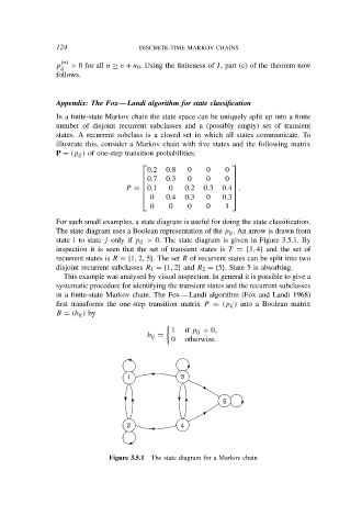
For such small examples, a state diagram is useful for doing the state classification.
The state diagram uses a Boolean representation of the p ij . An arrow is drawn from
state i to state j only if p ij > 0. The state diagram is given in Figure 3.5.1. By
inspection it is seen that the set of transient states is T = {3, 4} and the set of
recurrent states is R = {1, 2, 5}. The set R of recurrent states can be split into two
disjoint recurrent subclasses R 1 = {1, 2} and R 2 = {5}. State 5 is absorbing.
This example was analysed by visual inspection. In general it is possible to give a
systematic procedure for identifying the transient states and the recurrent subclasses
in a finite-state Markov chain. The Fox—Landi algorithm (Fox and Landi 1968)
first transforms the one-step transition matrix P = (p ij ) into a Boolean matrix
B = (b ij ) by

1 if p ij > 0,
b ij =
0 otherwise.

1 3

5

2 4

Figure 3.5.1 The state diagram for a Markov chain