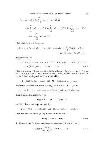
Page 166 - A First Course In Stochastic Models

MARKOV PROCESSES ON A SEMI-INFINITE STRIP 159

∞
i
(λ s + µ s + β s + δ s ) p(i, s)z − µ s p(0, s)
i=0
∞ ∞ ∞

i i i
= λ s p(i − 1, s)z + µ s p(i + 1, s)z + β s−1 p(i, s − 1)z
i=1 i=0 i=0
∞
i
+ δ s+1 p(i, s + 1)z .
i=0
This gives for s = 0, 1, . . . , m,

µ s
(λ s + µ s + β s + δ s )G s (z) − µ s p(0, s) = λ s zG s (z) + [G s (z) − p(0, s)]
z
+ β s−1 G s−1 (z) + δ s+1 G s+1 (z).

We rewrite this as
2
[λ s z + µ s − (λ s + µ s + β s + δ s )z]G s (z) + β s−1 zG s−1 (z) + δ s+1 zG s+1 (z)
= µ s (1 − z)p(0, s), s = 0, 1, . . . , m. (4.4.5)
This is a system of linear equations in the unknowns G 0 (z), . . . , G m (z). To see
what the solution looks like, it is convenient to write (4.4.5) in matrix notation. To
do so, define the diagonal matrices and M by

= diag(λ 0 , λ 1 , . . . , λ m ) and M = diag(µ 0 , µ 1 , . . . , µ m ).

Define the transition rate matrix T = (t ab ) with a, b = 0, 1, . . . , m by
t s,s−1 = β s−1 , t s,s+1 = δ s+1 , t ss = −(β s + δ s ) and t ab = 0 otherwise.

Finally, define the matrix A(z) by
2
A(z) = z − ( − T + M)z + M

and the column vectors p 0 and g(z) by
p 0 = (p(0, 0), . . . , p(0, m)) and g(z) = (G 0 (z), . . . , G m (z)).

Then the linear equations (4.4.5) in matrix notation are

A(z)g(z) = (1 − z)Mp 0 (4.4.6)
By Cramer’s rule for linear equations, the solution of (4.4.6) is given by

det A s (z)
G s (z) = , s = 0, 1, . . . , m, (4.4.7)
det A(z)