Page 167 - A First Course In Stochastic Models

160 CONTINUOUS-TIME MARKOV CHAINS

where A s (z) is the matrix that results from replacing the (s + 1)th column vec-
tor of A(z) by the vector (1 − z)Mp . The functions det A s (z) and det A(z) are
0
polynomials in z and are thus defined on the whole complex plane. Assuming that
the function N(z) = det A(z) satisfies the conditions stated in Theorem C.1 in
Appendix C, the representation (4.4.7) implies the following result.
Theorem 4.4.1 For each s = 0, 1, . . . , m, there is a constant γ s such that

i
p(i, s) ∼ γ s η as i → ∞, (4.4.8)
where η is the reciprocal of the smallest root of the equation
det A(x) = 0 (4.4.9)

on the interval (1, ∞).
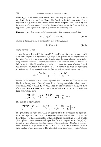
How do we solve (4.4.9) in general? A possible way is to use a basic result
from linear algebra stating that det A(x) equals the product of the eigenvalues of
the matrix A(x). It is a routine matter to determine the eigenvalues of a matrix by
using standard software. A search procedure such as bisection can next be used to
find the root of (4.4.9). Another approach to compute the roots of det A(z) = 0
was proposed in Chapter 3 of Daigle (1991). The zeros of det A(z) are equivalent
to the inverses of the eigenvalues of the 2(m + 1)-dimensional square matrix
−1 −1
M ( − T + M) −M
A E = ,
I O
where O is the matrix with all entries equal to zero. Note that M −1 exists. To see
this, let σ be any zero of det A(z) and let x σ be any non-trivial column vector
such that A(σ)x σ = 0. Let y σ = σx σ . Then, by the definition of A(z), we have
2
σ x σ −σ( − T + M)x +Mx σ = 0. By definition, y σ −σx σ = 0. Combining
σ
these two systems gives

M O − T + M − x σ
− σ = 0.
O I I O y σ
This system is equivalent to

−1 −1
M ( − T + M) −M 1 I O x σ
− = 0.
I O σ O I y σ
This proves that the zeros of det A(z) are equivalent to the inverses of the eigenval-
ues of the expanded matrix A E . The largest of the eigenvalues in (0, 1) gives the
decay factor η of the geometric tail of the equilibrium probabilities p(i, s). Daigle
(1991) gives a more sophisticated algorithm for the computation of the p(i, s).
Using the eigenvalues and the eigenvectors of the matrix A E , this algorithm com-
putes for each s the probabilities p(i, s) for i ≥ 1 as a linear combination of a
finite number of geometric terms. The interested reader is referred to Daigle’s book