Page 185 - A First Course In Stochastic Models

178 CONTINUOUS-TIME MARKOV CHAINS

and

f (τ, r) = 0 for any τ ≥ 0 when r < 0.
j
Using the simple-minded approximation

x x/ −1

f j (t, y) dy ≈ f (t, ℓ ) ,
j
0
ℓ=0
the desired probability P {R(t) ≤ x} is approximated by
x/ −1

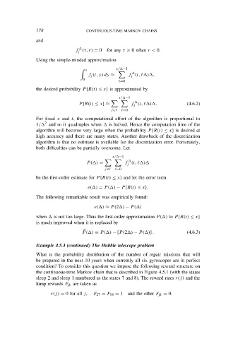
P {R(t) ≤ x} ≈ f (t, ℓ ) . (4.6.2)
j
j∈I ℓ=0
For fixed x and t, the computational effort of the algorithm is proportional to
2
1/ and so it quadruples when is halved. Hence the computation time of the
algorithm will become very large when the probability P {R(t) ≤ x} is desired at
high accuracy and there are many states. Another drawback of the discretization
algorithm is that no estimate is available for the discretization error. Fortunately,
both difficulties can be partially overcome. Let

x/ −1

P ( ) = f (t, ℓ )
j
j∈I ℓ=0
be the first-order estimate for P {R(t) ≤ x} and let the error term
e( ) = P ( ) − P {R(t) ≤ x}.

The following remarkable result was empirically found:
e( ) ≈ P (2 ) − P ( )

when is not too large. Thus the first-order approximation P ( ) to P {R(t) ≤ x}
is much improved when it is replaced by

P ( ) = P ( ) − [P (2 ) − P ( )] . (4.6.3)

Example 4.5.3 (continued) The Hubble telescope problem
What is the probability distribution of the number of repair missions that will
be prepared in the next 10 years when currently all six gyroscopes are in perfect
condition? To consider this question we impose the following reward structure on
the continuous-time Markov chain that is described in Figure 4.5.1 (with the states
sleep 2 and sleep 1 numbered as the states 7 and 8). The reward rates r(j) and the
lump rewards F jk are taken as
r(j) = 0 for all j, F 27 = F 18 = 1 and the other F jk = 0.