Page 181 - A First Course In Stochastic Models

174 CONTINUOUS-TIME MARKOV CHAINS

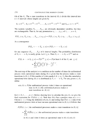
kth of the U i . The n state transitions in the interval (0, t) divide this interval into
n + 1 intervals whose lengths are given by

(1) (2) (1) (n) (n−1) (n)
Y 1 = U , Y 2 = U − U , . . . , Y n = U − U and Y n+1 = t − U .

The random variables Y 1 , . . . , Y n+1 are obviously dependent variables, but they
are exchangeable. That is, for any permutation i 1 , . . . , i n+1 of 1, . . . , n + 1,

≤ x n+1 } = P {Y 1 ≤ x 1 , Y 2 ≤ x 2 , . . ., Y n+1 ≤ x n+1 }.
P {Y i 1 ≤x 1 , Y i 2 ≤x 2 , . . ., Y i n+1

As a consequence

P {Y i 1 + · · · + Y i k ≤ x} = P {Y 1 + · · · + Y k ≤ x}
) of k interval lengths. The probability distribution
for any sequence (Y i 1 , . . . , Y i k
of Y 1 + · · · + Y k is easily given. Let k ≤ n. Then Y 1 + · · · + Y k = U (k) and so

P {Y 1 + · · · + Y k ≤ x} = P {U (k) ≤ x} = P {at least k of the U i are ≤ x}
x j
n
n x n−j

= 1 − .
j t t
j=k
The next step of the analysis is to condition on the number of times the uniformized
process visits operational states during (0, t) given that the process makes n state
transitions in (0, t). If this number of visits equals k (k ≤ n+1), then the cumulative
operational time during (0, t) is distributed as Y 1 + · · · + Y k . For any given n ≥ 0,
define
α(n, k) = P {the uniformized process visits k times an operational
state in (0, t) | the uniformized process makes n
state transitions in (0, t)}
for k = 0, 1, . . . , n + 1. Before showing how to calculate the α(n, k), we give the
final expression for P {O(t) ≤ x}. Note that O(t) has a positive mass at x = t.
Choose x < t. Using the definition of α(n, k) and noting that O(t) ≤ x only if the
uniformized process visits at least one non-operational state in (0, t), it follows that

P {O(t) ≤ x | the uniformized processes makes n state transitions in (0, t)}
n

= P {O(t) ≤ x | the uniformized process makes n state transitions
k=0
in (0, t) and visits k times an operational state in (0, t)} α(n, k)