Page 28 - A First Course In Stochastic Models

COMPOUND POISSON PROCESSES 19

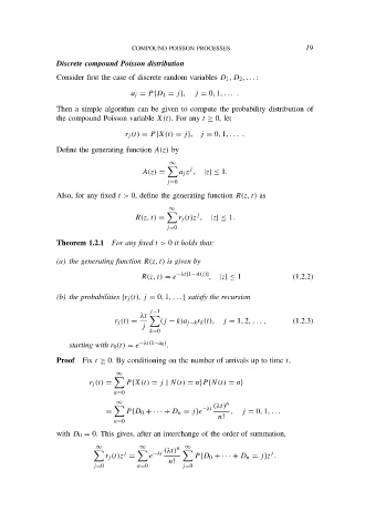
Discrete compound Poisson distribution
Consider first the case of discrete random variables D 1 , D 2 , . . . :

a j = P {D 1 = j}, j = 0, 1, . . . .
Then a simple algorithm can be given to compute the probability distribution of
the compound Poisson variable X(t). For any t ≥ 0, let
r j (t) = P {X(t) = j}, j = 0, 1, . . . .

Define the generating function A(z) by
∞
j
A(z) = a j z , |z| ≤ 1.
j=0
Also, for any fixed t > 0, define the generating function R(z, t) as

∞
j
R(z, t) = r j (t)z , |z| ≤ 1.
j=0
Theorem 1.2.1 For any fixed t > 0 it holds that:

(a) the generating function R(z, t) is given by
R(z, t) = e −λt{1−A(z)} , |z| ≤ 1 (1.2.2)

(b) the probabilities {r j (t), j = 0, 1, . . . } satisfy the recursion
j−1
λt
r j (t) = (j − k)a j−k r k (t), j = 1, 2, . . . , (1.2.3)
j
k=0
starting with r 0 (t) = e −λt(1−a 0 ) .
Proof Fix t ≥ 0. By conditioning on the number of arrivals up to time t,
∞

r j (t) = P {X(t) = j | N(t) = n}P {N(t) = n}
n=0
∞ n
−λt (λt)
= P {D 0 + · · · + D n = j}e , j = 0, 1, . . .
n!
n=0
with D 0 = 0. This gives, after an interchange of the order of summation,
∞ ∞ n ∞
j −λt j
(λt)
r j (t)z = e P {D 0 + · · · + D n = j}z .
n!
j=0 n=0 j=0