Page 30 - A First Course In Stochastic Models

COMPOUND POISSON PROCESSES 21

scheme for computing Poisson probabilities. An alternative method to compute the
compound Poisson probabilities r j (t), j = 0, 1, . . . is to apply the discrete FFT
method to the explicit expression (1.2.2) for the generating function of the r j (t);
see Appendix D.

Continuous compound Poisson distribution
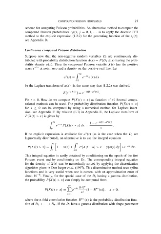
Suppose now that the non-negative random variables D i are continuously dis-
tributed with probability distribution function A(x) = P {D 1 ≤ x} having the prob-
ability density a(x). Then the compound Poisson variable X(t) has the positive
mass e −λt at point zero and a density on the positive real line. Let

∞
∗ −sx
a (s) = e a(x) dx
0
be the Laplace transform of a(x). In the same way that (1.2.2) was derived,
∗
E[e −sX(t) ] = e −λt{1−a (s)} .
Fix t > 0. How do we compute P {X(t) > x} as function of x? Several compu-
tational methods can be used. The probability distribution function P {X(t) > x}
for x ≥ 0 can be computed by using a numerical method for Laplace inver-
sion; see Appendix F. By relation (E.7) in Appendix E, the Laplace transform of
P {X(t) > x} is given by

∗
∞ 1 − e −λt{1−a (s)}

e −sx P {X(t) > x} dx = .
0 s
If no explicit expression is available for a (s) (as is the case when the D i are
∗
lognormally distributed), an alternative is to use the integral equation
t
x
P {X(t) > x} = 1 − A(x) + P {X(t − u) > x − y}a(y) dy λe −λu du.
0 0
This integral equation is easily obtained by conditioning on the epoch of the first
Poisson event and by conditioning on D 1 . The corresponding integral equation
for the density of X(t) can be numerically solved by applying the discretization
algorithm given in Den Iseger et al. (1997). This discretization method uses spline
functions and is very useful when one is content with an approximation error of
about 10 −8 . Finally, for the special case of the D i having a gamma distribution,
the probability P {X(t) > x} can simply be computed from
∞ n
−λt (λt)
n∗
P {X(t) > x} = e {1 − B (x)}, x > 0,
n!
n=1
where the n-fold convolution function B n∗ (x) is the probability distribution func-
tion of D 1 + · · · + D n . If the D i have a gamma distribution with shape parameter