Page 306 - A First Course In Stochastic Models

300 SEMI-MARKOV DECISION PROCESSES

EXERCISES
7.1 Consider a production facility that operates only intermittently to manufacture a single
product. The production will be stopped if the inventory is sufficiently high, whereas the
production will be restarted when the inventory has dropped sufficiently low. Customers
asking for the product arrive according to a Poisson process with rate λ. The demand of
each customer is for one unit. Demand which cannot be satisfied directly from stock on
hand is lost. Also, a finite capacity C for the inventory is assumed. In a production run, any
desired lot size can be produced. The production time of a lot size of Q units is a random
variable T Q having a probability density f Q (t). The lot size is added to the inventory at the
end of the production run. After the completion of a production run, a new production run is
started or the facility is closed down. At each point of time the production can be restarted.
The production costs for a lot size of Q ≥ 1 units consist of a fixed set-up cost K > 0 and
a variable cost c per unit produced. Also, there is a holding cost of h > 0 per unit kept in
stock per time unit, and a lost-sales cost of p > 0 is incurred for each lost demand. The
goal is to minimize the long-run average cost per time unit. Formulate the problem as a
semi-Markov decision model.
7.2 Consider the maintenance problem from Example 6.1.1 again. The numerical data are
given in Table 6.4.1. Assume now that a repair upon failure takes either 1, 2 or 3 days,
each with probability 1/3. Use the semi-Markov model to compute by policy iteration or
linear programming an average cost optimal policy. Can you explain why you get the same
optimal policy as in Example 6.1.1?
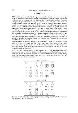
7.3 A cargo liner operates between the five harbours A 1 , . . . , A 5 . A cargo shipment from
harbour A i to harbour A j (j = i) takes a random number τ ij of days (including load and
discharge) and yields a random pay-off of ξ ij . The shipment times τ ij and the pay-offs ξ ij
are normally distributed with means µ(τ ij ) and µ(ξ ij ) and standard deviations σ(τ ij ) and
σ(ξ ij ). We assume the numerical data:

µ(τ ij )[σ(τ ij )]
i\j 1 2 3 4 5

1
1
1
1 - 3 6 [1] 3 2
2 2 2

2 4 [1] - 1 1 7 [1] 5 [1]
4

3 5 [1] 1 1 - 6 [1] 8 [1]
4

4 3 1 8 [1] 5 [1] - 2 1
2 2
1

1
5 2 5 [1] 9 [1] 2 -
2 2
µ(ξ ij )[σ(ξ ij )]
i\j 1 2 3 4 5
1 - 8 [1] 12 [2] 6 [1] 6 [1]

1
2 20 [3] - 2 14 [3] 16 [2]
2

3 16 [3] 2 1 - 18 [3] 16 [1]
2

4 6 [1] 10 [2] 20 [2] - 6 1
2
5 8 [2] 16 [3] 20 [2] 8 [1] -
Compute by policy iteration or linear programming a sailing route for which the long-run
average reward per day is maximal.