Page 305 - A First Course In Stochastic Models

ONE-STEP POLICY IMPROVEMENT 299

for T s+1 and K s+1 into (7.5.3) and (7.5.4) with i = s, we get two systems of linear
equations for T i , 1 ≤ i ≤ s and K i , 1 ≤ i ≤ s. Once these systems of linear
equations have been solved, we can next compute T i and K i for any desired i > s.
Summarizing, the heuristic algorithm proceeds as follows.

Heuristic algorithm
(0)
Step 1. Compute the best values p , k = 1, . . . , n, of the Bernoulli-splitting
k
probabilities by minimizing the expression (7.5.1) subject to n p k = 1 and
k=1
0 ≤ λp k < s k µ k for k = 1, . . . , n.
Step 2. For each queue k = 1, . . . , n, solve the system of linear equations (7.5.3)
(0)
and (7.5.4) with α = λp , s = s k and µ = µ k . Next compute for each queue k
k
(0)
the function w k (i) from (7.5.2) with α = λp , s = s k and µ = µ k .
k
Step 3. For each state x = (i 1 , . . . , i n ), determine an index k 0 achieving the mini-
mum in
min {w k (i k + 1) − w k (i k )}.
1≤k≤n
The separable rule assigns a new arrival in state x = (i 1 , . . . , i n ) to queue k 0 .
Numerical results
Let us consider the numerical data

s 1 = 10, s 2 = 1, µ 1 = 1 and µ 2 = 9.
The traffic load ρ, which is defined by

ρ = λ/(s 1 µ 1 + s 2 µ 2 ),
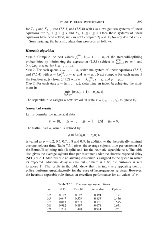
is varied as ρ = 0.2, 0.5, 0.7, 0.8 and 0.9. In addition to the theoretically minimal
average sojourn time, Table 7.5.1 gives the average sojourn time per customer for
the Bernoulli-splitting rule (B-split) and for the heuristic separable rule. The table
also gives the average sojourn time per customer under the shortest expected delay
(SED) rule. Under this rule an arriving customer is assigned to the queue in which
its expected individual delay is smallest (if there is a tie, the customer is sent
to queue 1). The results in the table show that this intuitively appealing control
policy performs unsatisfactorily for the case of heterogeneous services. However,
the heuristic separable rule shows an excellent performance for all values of ρ.

Table 7.5.1 The average sojourn times
ρ SED B-split Separable Optimal
0.2 0.192 0.192 0.191 0.191
0.5 0.647 0.579 0.453 0.436
0.7 0.883 0.737 0.578 0.575
0.8 0.982 0.897 0.674 0.671
0.9 1.235 1.404 0.941 0.931