Page 317 - A First Course In Stochastic Models

312 ADVANCED RENEWAL THEORY

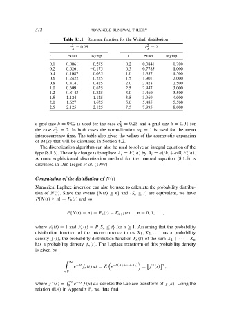
Table 8.1.1 Renewal function for the Weibull distribution
2 2
c = 0.25 c = 2
X X
t exact asymp t exact asymp
0.1 0.0061 −0.275 0.2 0.3841 0.700
0.2 0.0261 −0.175 0.5 0.7785 1.000
0.4 0.1087 0.025 1.0 1.357 1.500
0.6 0.2422 0.225 1.5 1.901 2.000
0.8 0.4141 0.425 2.0 2.428 2.500
1.0 0.6091 0.625 2.5 2.947 3.000
1.2 0.8143 0.825 3.0 3.460 3.500
1.5 1.124 1.125 3.5 3.969 4.000
2.0 1.627 1.625 5.0 5.485 5.500
2.5 2.125 2.125 7.5 7.995 8.000

2
a grid size h = 0.02 is used for the case c = 0.25 and a grid size h = 0.01 for
X
the case c 2 = 2. In both cases the normalization µ 1 = 1 is used for the mean
X
interoccurrence time. The table also gives the values of the asymptotic expansion
of M(x) that will be discussed in Section 8.2.
The discretization algorithm can also be used to solve an integral equation of the
type (8.1.5). The only change is to replace A i = F(ih) by A i = a(ih)+a(0)F(ih).
A more sophisticated discretization method for the renewal equation (8.1.5) is
discussed in Den Iseger et al. (1997).

Computation of the distribution of N(t)
Numerical Laplace inversion can also be used to calculate the probability distribu-
tion of N(t). Since the events {N(t) ≥ n} and {S n ≤ t} are equivalent, we have
P {N(t) ≥ n} = F n (t) and so

P {N(t) = n} = F n (t) − F n+1 (t), n = 0, 1, . . . ,

where F 0 (t) = 1 and F n (t) = P {S n ≤ t} for n ≥ 1. Assuming that the probability
distribution function of the interoccurrence times X 1 , X 2 , . . . has a probability
density f (t), the probability distribution function F n (t) of the sum X 1 + · · · + X n
has a probability density f n (t). The Laplace transform of this probability density
is given by

∞ −st −s(X 1 +···+X n )
n

∗
e f n (t) dt = E e = f (s) ,
0
∞ −sx
∗
where f (s) = e f (x) dx denotes the Laplace transform of f (x). Using the
0
relation (E.4) in Appendix E, we thus find