Page 358 - A First Course In Stochastic Models

THE M/G/1 QUEUE 353

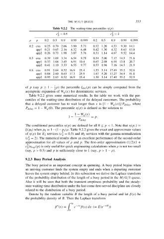
Table 9.2.2 The waiting-time percentiles η(p)
2
2
c = 0.5 c = 2
S S
ρ p 0.2 0.5 0.9 0.99 0.999 0.2 0.5 0.9 0.99 0.999
0.2 exa 0.25 0.70 2.06 3.90 5.73 0.32 1.20 4.53 9.30 14.1
app1 0.21 0.65 2.16 4.32 6.48 0.42 1.30 4.32 8.63 13.0
app2 0.26 0.73 1.98 3.87 5.76 0.31 1.14 4.67 9.52 14.4
0.5 exa 0.39 1.09 3.34 6.54 9.75 0.54 2.00 7.12 14.5 21.8
app1 0.33 1.04 3.45 6.91 10.4 0.67 2.08 6.91 13.8 20.7
app2 0.41 1.10 3.33 6.55 9.77 0.53 1.96 7.16 14.5 21.9
0.8 exa 0.91 2.64 8.52 16.9 25.4 1.53 5.14 17.49 35.2 52.8
app1 0.84 2.60 8.63 17.3 25.9 1.67 5.20 17.27 34.5 51.8
app2 0.93 2.63 8.52 16.9 25.4 1.50 5.14 17.49 35.2 52.9

1
of p (say p ≥ 1 − ρ) the percentile ξ det (p) can be simply computed from the
2
asymptotic expansion of W q (x) for deterministic services.
Table 9.2.2 gives some numerical results. In the table we work with the per-
centiles of the waiting-time distribution of the delayed customers. The probability
that a delayed customer has to wait longer than x is [1 − W q (x)]/P delay , where
P delay = 1 − W q (0). The percentile η(p) is defined as the solution to

1 − W q (x)
1 − = p.
P delay
The conditional percentiles η(p) are defined for all 0 ≤ p < 1. Note that η(p 1 ) =
ξ(p 0 ) when p 0 = 1−(1−p 1 )ρ. Table 9.2.2 gives the exact and approximate values
2
of η(p) for E 2 services (c = 0.5) and H 2 services with the gamma normalization
S
2
(c = 2). The numerical results show an excellent performance of the second-order
S
approximation for all values of ρ and p. The first-order approximation (1/2)(1 +
2
c )η exp (p) is only useful for quick engineering calculations when ρ is not too small
S
(say, ρ > 0.5) and p is sufficiently close to 1 (say, p > 1 − ρ).
9.2.3 Busy Period Analysis
The busy period is an important concept in queueing. A busy period begins when
an arriving customer finds the system empty and ends when a departing customer
leaves the system empty behind. In this subsection we derive the Laplace transform
of the probability distribution of the length of a busy period in the M/G/1 queue.
Also it will be seen that both the transient emptiness probability and the steady-
state waiting-time distribution under the last-come first-served discipline are closely
related to the distribution of a busy period.
Denote by the random variable B the length of a busy period and let β(x) be
the probability density of B. Then the Laplace transform
∞

∗ −sx −sB
β (s) = e β(x) dx (= E(e ))
0