Page 470 - A First Course In Stochastic Models

F. NUMERICAL LAPLACE INVERSION 465

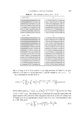
Table F.1 The constants α j and λ j for n = 8, 16
α j (n = 8) λ j
2.00000000000000000000E+00 3.14159265358979323846E+00
2.00000000000009194165E+00 9.42477796076939341796E+00
2.00000030233693694331E+00 1.57079633498486685135E+01
2.00163683400961269435E+00 2.19918840702852034226E+01
2.19160665410378500033E+00 2.84288098692614839228E+01
4.01375304677448905244E+00 3.74385643171158002866E+01
1.18855502586988811981E+01 5.93141454252504427542E+01
1.09907452904076203170E+02 1.73674723843715552399E+02
α j (n = 16) λ j
2.00000000000000000000E+00 3.14159265358979323846E+00
2.00000000000000000000E+00 9.42477796076937971539E+00
2.00000000000000000000E+00 1.57079632679489661923E+01
2.00000000000000000000E+00 2.19911485751285526692E+01
2.00000000000000025539E+00 2.82743338823081392079E+01
2.00000000001790585116E+00 3.45575191894933477513E+01
2.00000009630928117646E+00 4.08407045355964511919E+01
2.00006881371091937456E+00 4.71239261219868564304E+01
2.00840809734614010315E+00 5.34131955661131603664E+01
2.18638923693363504375E+00 5.99000285454941069650E+01
3.03057284932114460466E+00 6.78685456453781178352E+01
4.82641532934280440182E+00 7.99199036559694718061E+01
8.33376254184457094255E+00 9.99196221424608443952E+01
1.67554002625922470539E+01 1.37139145843604237972E+02
4.72109360166038325036E+01 2.25669154692295029965E+02
4.27648046755977518689E+02 6.72791727521303673697E+02

take n as large as 8 or 16 to achieve a very high precision. In Table F.1 we give
both for n = 8 and n = 16 the abscissae λ j and the weights α j for j = 1, . . . , n.
It is convenient to rewrite (F.2) as

n 2
e bℓ b + iλ j + iπ(t − 1)
f (ℓ ) ≈ α j Re f ∗ cos(πℓt) dt.
0
j=1

# $
1
n 2 ∗ b+iλ j +iπ(t−1)
Put for abbreviation g ℓ = α Re f cos(πℓt) dt. Then
2 j=1 j 0
bℓ
f (ℓ ) ≈ (2e / )g ℓ . The integral in g ℓ is calculated by using the trapezoidal rule
approximation with a division of the integration interval (0, 2) into 2m subintervals
of length 1/m for an appropriately chosen value of m. It is recommended to take
m = 4M. This gives
2m−1
∗
∗
1 πℓp f + f 2m
0
∗
g ℓ ≈ f cos + , (F.3)
p
2m m 2
p=1