Page 473 - A First Course In Stochastic Models

468 APPENDICES

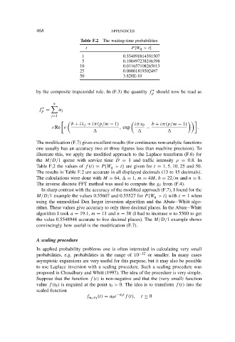
Table F.2 The waiting-time probabilities
t P{W q > t}
1 0.554891814301507
5 0.100497238246398
10 0.011657108265013
25 0.00001819302497
50 3.820E-10

∗
by the composite trapezoidal rule. In (F.3) the quantity f should now be read as
p
n

∗
f = α j
p
j=1
b + iλ j + iπ(p/m − 1) iπx 0 b + iπ(p/m − 1)

×Re v , exp − .

The modification (F.7) gives excellent results (for continuous non-analytic functions
one usually has an accuracy two or three figures less than machine precision). To
illustrate this, we apply the modified approach to the Laplace transform (F.6) for
the M/D/1 queue with service time D = 1 and traffic intensity ρ = 0.8. In
Table F.2 the values of f (t) = P {W q > t} are given for t = 1, 5, 10, 25 and 50.
The results in Table F.2 are accurate in all displayed decimals (13 to 15 decimals).
The calculations were done with M = 64, = 1, m = 4M, b = 22/m and n = 8.
The inverse discrete FFT method was used to compute the g ℓ from (F.4).
In sharp contrast with the accuracy of the modified approach (F.7), I found for the
M/D/1 example the values 0.55607 and 0.55527 for P {W q > t} with t = 1 when
using the unmodified Den Iseger inversion algorithm and the Abate–Whitt algo-
rithm. These values give accuracy to only three decimal places. In the Abate–Whitt
algorithm I took a = 19.1, m = 11 and n = 38 (I had to increase n to 5500 to get
the value 0.5548948 accurate to five decimal places). The M/D/1 example shows
convincingly how useful is the modification (F.7).

A scaling procedure
In applied probability problems one is often interested in calculating very small
probabilities, e.g. probabilities in the range of 10 −12 or smaller. In many cases
asymptotic expansions are very useful for this purpose, but it may also be possible
to use Laplace inversion with a scaling procedure. Such a scaling procedure was
proposed in Choudhury and Whitt (1997). The idea of the procedure is very simple.
Suppose that the function f (t) is non-negative and that the (very small) function
value f (t 0 ) is required at the point t 0 > 0. The idea is to transform f (t) into the
scaled function
(t) = a 0 e −a 1 t f (t), t ≥ 0
f a 0 ,a 1