Page 478 - A First Course In Stochastic Models

G. THE ROOT-FINDING PROBLEM 473

c
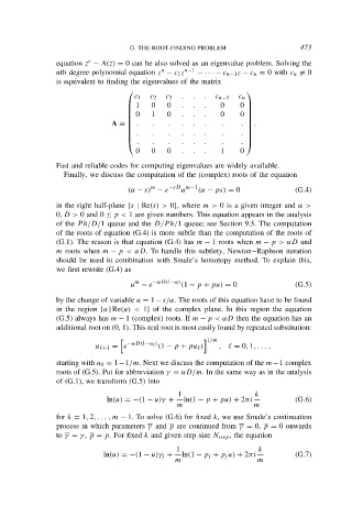
equation z − A(z) = 0 can be also solved as an eigenvalue problem. Solving the
n
nth degree polynomial equation z − c 1 z n−1 − · · · − c n−1 z − c n = 0 with c n = 0
is equivalent to finding the eigenvalues of the matrix
 
c 1 c 2 c 3 . . . c n−1 c n
1 0 0 0 0
 . . . 
 
0 1 0 0 0
 . . . 
 
A =  . . . . . . . .  .
 
. . . . . . . .
 
 
 . . . . . . . . 
0 0 0 . . . 1 0
Fast and reliable codes for computing eigenvalues are widely available.
Finally, we discuss the computation of the (complex) roots of the equation
m −sD m−1
(α − s) − e α (α − ps) = 0 (G.4)
in the right half-plane {s | Re(s) > 0}, where m > 0 is a given integer and α >
0, D > 0 and 0 ≤ p < 1 are given numbers. This equation appears in the analysis
of the P h/D/1 queue and the D/P h/1 queue; see Section 9.5. The computation
of the roots of equation (G.4) is more subtle than the computation of the roots of
(G.1). The reason is that equation (G.4) has m − 1 roots when m − p > αD and
m roots when m − p < αD. To handle this subtlety, Newton–Raphson iteration
should be used in combination with Smale’s homotopy method. To explain this,
we first rewrite (G.4) as
m
u − e −αD(1−u) (1 − p + pu) = 0 (G.5)
by the change of variable u = 1−s/α. The roots of this equation have to be found
in the region {u | Re(u) < 1} of the complex plane. In this region the equation
(G.5) always has m − 1 (complex) roots. If m − p < αD then the equation has an
additional root on (0, 1). This real root is most easily found by repeated substitution:
1/m

u ℓ+1 = e −αD(1−u ℓ ) (1 − p + pu ℓ ) , ℓ = 0, 1, . . . ,
starting with u 0 = 1−1/m. Next we discuss the computation of the m−1 complex
roots of (G.5). Put for abbreviation γ = αD/m. In the same way as in the analysis
of (G.1), we transform (G.5) into
1 k
ln(u) = −(1 − u)γ + ln(1 − p + pu) + 2πi (G.6)
m m
for k = 1, 2, . . . , m − 1. To solve (G.6) for fixed k, we use Smale’s continuation
process in which parameters γ and p are continued from γ = 0, p = 0 onwards
to γ = γ , p = p. For fixed k and given step size N step , the equation
1 k
ln(u) = −(1 − u)γ j + ln(1 − p j + p j u) + 2πi (G.7)
m m