Page 86 - A First Course In Stochastic Models

EXERCISES 77

exponentially distributed time with mean 1/ν. If the server is idle, the customer gets served,
otherwise the customer returns to orbit and tries again after an exponentially distributed time
until the server is found free. The customers in orbit act independently of each other. The
service times of the customers are independent random variables having the same general
probability distribution. Letting the random variable S denote the service time of a customer,
it is assumed that ρ = λE(S) is less than 1. For this model, known as the M/G/1 queue
with retrials, define L(t) as the number of customers in the system (service station plus
orbit) at time t and define Q n as the number of customers in orbit just after the nth service
completion. Let p j = lim t→∞ P{L(t) = j} and q j = lim n→∞ P{Q n = j} for j ≥ 0.
(a) Use an up- and downcrossing argument to argue that p j = q j for all j ≥ 0.
q
∞ j
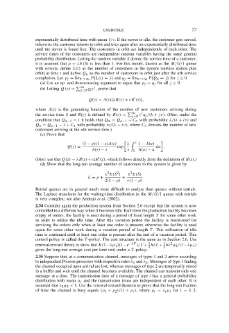
(b) Letting Q (z) = j=0 j z , prove that
Q(z) = A(z){λR(z) + νR (z)},
′
where A(z) is the generating function of the number of new customers arriving during
∞
j
the service time S and R(z) is defined by R(z) = z q j /(λ + jν). (Hint: under the
j=0
condition that Q n−1 = i it holds that Q n = Q n−1 + C n with probability λ/(λ + iν) and
Q n = Q n−1 − 1 + C n with probability iν/(λ + iν), where C n denotes the number of new
customers arriving at the nth service time.)
(c) Prove that
λ
(1 − ρ)(1 − z)A(z) z 1 − A(u)
Q(z) = exp du .
A(z) − z ν 1 A(u) − u
(Hint: use that Q(z) = λR(z)+νzR (z), which follows directly from the definition of R(z).)
′
(d) Show that the long-run average number of customers in the system is given by
2
2
2
λ E(S ) λ E(S)
L = ρ + + .
2(1 − ρ) ν(1 − ρ)
Retrial queues are in general much more difficult to analyse than queues without retrials.
The Laplace transform for the waiting-time distribution in the M/G/1 queue with retrials
is very complex; see also Artalejo et al. (2002).
2.34 Consider again the production system from Section 2.6 except that the system is now
controlled in a different way when it becomes idle. Each time the production facility becomes
empty of orders, the facility is used during a period of fixed length T for some other work
in order to utilize the idle time. After this vacation period the facility is reactivated for
servicing the orders only when at least one order is present; otherwise the facility is used
again for some other work during a vacation period of length T . This utilization of idle
time is continued until at least one order is present after the end of a vacation period. This
control policy is called the T -policy. The cost structure is the same as in Section 2.6. Use
1
1
2
renewal-reward theory to show that K(1−λµ 1 )(1−e −λT )/T + hλT + hλ µ 2 /(1−λµ 1 )
2
2
gives the long-run average cost per time unit under a T -policy.
2.35 Suppose that, at a communication channel, messages of types 1 and 2 arrive according
to independent Poisson processes with respective rates λ 1 and λ 2 . Messages of type 1 finding
the channel occupied upon arrival are lost, whereas messages of type 2 are temporarily stored
in a buffer and wait until the channel becomes available. The channel can transmit only one
message at a time. The transmission time of a message of type i has a general probability
distribution with mean µ i and the transmission times are independent of each other. It is
assumed that λ 2 µ 2 < 1. Use the renewal-reward theorem to prove that the long-run fraction
of time the channel is busy equals (ρ 1 + ρ 2 )/(1 + ρ 1 ), where ρ i = λ i µ i for i = 1, 2.