Page 93 - A First Course In Stochastic Models

THE MODEL 85

Example 3.1.2 A stock-control problem
The Johnson hardware shop carries adjustable-joint pliers as a regular stock item.
The demand for this tool is stable over time. The total demand during a week
has a Poisson distribution with mean λ. The demands in the successive weeks are
independent of each other. Each demand that occurs when the shop is out of stock
is lost. The owner of the shop uses a so-called periodic review (s, S) control rule
for stock replenishment of the item. The inventory position is only reviewed at
the beginning of each week. If the stock on hand is less than the reorder point s,
the inventory is replenished to the order-up point S; otherwise, no ordering is
done. Here s and S are given integers with 0 ≤ s ≤ S. The replenishment time is
negligible. What is the average ordering frequency and what is the average amount
of demand that is lost per week?
These questions can be answered by the theory of Markov chains. In this example
we take as state variable the stock on hand just prior to review. Let
X n = the stock on hand at the beginning of the nth week just prior to review,

then the stochastic process {X n } is a discrete-time Markov chain with the finite
state space I = {0, 1, . . . , S}. It will be immediately clear that the Markovian
property (3.1.1) is satisfied: the stock on hand at the beginning of the current week
and the demand in the coming week determine the stock on hand at the beginning
of the next week. It is not relevant how the stock level fluctuated in the past. To
find the one-step transition probabilities p ij = P {X n+1 = j | X n = i} we have
to distinguish the cases i ≥ s and i < s. In the first case the stock on hand just
after review equals i, while in the second case the stock on hand just after review
equals S. For state i ≥ s, we have

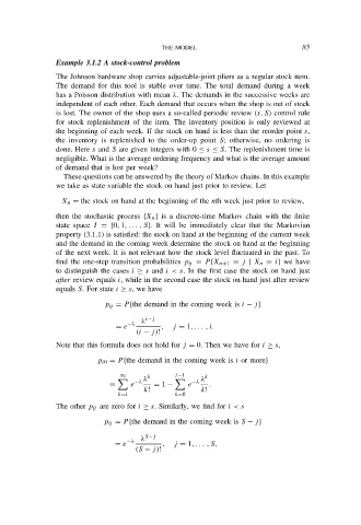
p ij = P {the demand in the coming week is i − j}
λ i−j
−λ
= e , j = 1, . . . , i.
(i − j)!
Note that this formula does not hold for j = 0. Then we have for i ≥ s,

p i0 = P {the demand in the coming week is i or more}

∞ k i−1 k
−λ λ −λ λ
= e = 1 − e .
k! k!
k=i k=0
The other p ij are zero for i ≥ s. Similarly, we find for i < s
p ij = P {the demand in the coming week is S − j}

λ S−j
−λ
= e , j = 1, . . . , S,
(S − j)!