Page 109 - A Guide to MATLAB for Beginners and Experienced Users

90 Practice Set B: Calculus, Graphics, and Linear Algebra

these numbers for large n and how they depend on the initial population.
Clearly

x n + y n + z n = 1, n ≥ 0.
Now we can use the table to express a relationship between the nthand
(n + 1)st generations. Because of our presumption on mating, only the first,
fourth, and sixth columns are relevant. Indeed a moment’s reflection re-
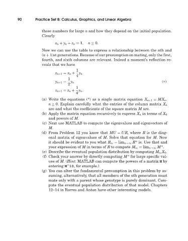
veals that we have
1
x n+1 = x n + y n
4
1
y n+1 = y n ( * )
2
1
z n+1 = z n + y n.
4
(a) Write the equations (*) as a single matrix equation X n+1 = MX n,
n ≥ 0. Explain carefully what the entries of the column matrix X n
are and what the coefficients of the square matrix M are.
(b) Apply the matrix equation recursively to express X n in terms of X 0
and powers of M.
(c) Next use MATLAB to compute the eigenvalues and eigenvectors of
M.
(d) From Problem 12 you know that MU = UR, where R is the diag-
onal matrix of eigenvalues of M. Solve that equation for M. Now
n
it should be evident to you what R ∞ = lim n→∞ R is. Use that and
n
your expression of M in terms of R to compute M ∞ = lim n→∞ M .
(e) Describe the eventual population distribution by computing M ∞ X 0 .
n
(f) Check your answer by directly computing M for large specific val-
ues of M.(Hint: MATLAB can compute the powers of a matrix M by
entering Mˆ10, for example.)
(g) You can alter the fundamental presumption in this problem by as-
suming, alternatively, that all members of the nthgeneration must
mate only witha parent whose genotype is purely dominant. Com-
pute the eventual population distribution of that model. Chapters
12–14 in Rorres and Anton have other interesting models.