Page 101 - A Practical Companion to Reservoir Stimulation

PRACTICAL COMPANION TO RESERVOIR STIMULATION

EXAMPLE F-9
Thus, from Eq. 11-14 the fracture half-length may be
Very Tight Oil Well- calculated.
Interpretation of Posttreatment Test
(4.064) ( 195) ( 1.3)
A very tight oil well was flowed above the bubblepoint for 60 xr' = (135)(47.4)
days and then was shut in for 50 days. The flow rate was 195
STB/d. A summary of the test is shown in Fig. F-4. The per- 0.3
meability, obtained from a pretreatment test, was 0.003 = 1380ft. (F-30)
md. Calculate the fracture geometry and conductivity. Table [(0.003)(0.09)(1.5 x
F-5 contains the relevant well and reservoir data. Sinje this fracture was designed for a kfw product equal
to 1300 md-ft, then
Solution (Ref. Section 11-6)
Figure F-5 is the log-log diagnostic plot for this test. Since the 1300 = 314, (F-3 I)
permeability is very low, it should be expected thatihe fracture FCD = (0.003) ( 1380)
conductivity should be very high (FcD > loo), and thus no
bilinear flow should be evident. Instead, linear flow, represented which readily justifies the appearance of linear flow and the
by the half-slope straight line on Fig. F-5, should denote the lack of bilinear flow.
large conductivity fracture. (In this test, the larger than 0.5
slope at later time is attributed to superposition effects. If the
buildup time is of the same order of duration as the flow time, I k = 0.003md I
e.g., 50 days, then distortion of the data can occur. Further I fo = 60days I
explanation of this trend is outside the scope of this example.) ~~
The linear flow trends lead to the specialized plot in Fig. @ = 0.09
F-6 where the square root of time vs. pressure is plotted on q = 195 STBId
I h = 135ft I
Cartesian coordinates. The slope is equal to 47.4 psi/hrO.'.

I Pwr = 3300psi I
ct = 1.5~ psi-'
r, = 0.328ft
€3, = 1.3 resbbl/STB

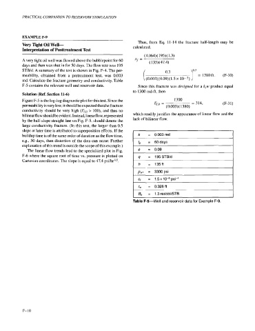
Table F-5-Well and reservoir data for Example F-9.

F- 10