Page 89 - A Course in Linear Algebra with Applications

3.2: Basic Properties of Determinants 73

which is turn equals the sum of

^2 •• ' kik ' ' ' a
a
signal,..., i n )oii 1
"3h ni n
and

c ^ s i g n ( i 1 , . . . , i n ) a i i l • • a 31 j a 3lk 1 a r

Now the first of these sums is simply det(^4), while the second
sum is the determinant of a matrix in which rows j and k are
identical, so it is zero by 3.2.2. Hence det(C) = det(A).

Now let us see how use of these properties can lighten the
task of evaluating a determinant. Let A be an n x n matrix
whose determinant is to be computed. Then elementary row
operations can be used as in Gaussian elimination to reduce A
to row echelon form B. But B is an upper triangular matrix,
say
(bn bi2 ••• & l n \
0 b 22 • • • b 2n
B =

\ 0 0 "nn /

so by 3.1.5 we obtain det(B) = 611622 • • -bun- Thus all that
has to be done is to keep track, using 3.2.3, of the changes in
det(.A) produced by the row operations.
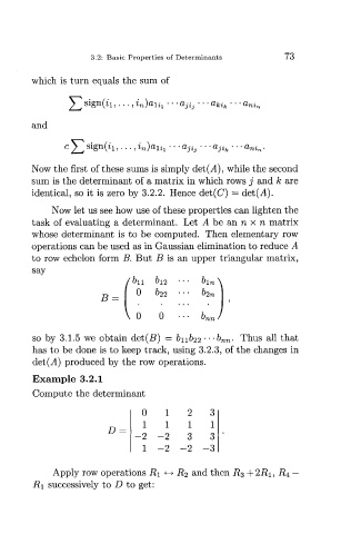
Example 3.2.1
Compute the determinant

0 1 2 3
1 1 1 1
D =
- 2 - 2 3 3
1 - 2 - 2 - 3

Apply row operations Ri <-» R 2 and then R 3 + 2R\, R4 —
i?i successively to D to get: