Page 209 - Adaptive Identification and Control of Uncertain Systems with Nonsmooth Dynamics

208 Adaptive Identification and Control of Uncertain Systems with Non-smooth Dynamics

equation
3

|sI − A|= (s − p i ) (13.15)
i=1
where I is the unit matrix.
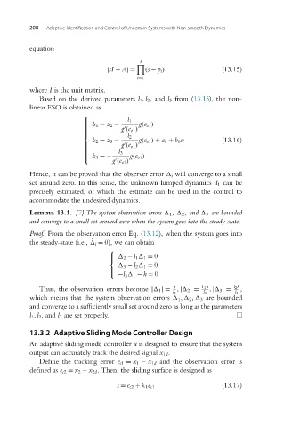
Based on the derived parameters l 1 ,l 2,and l 3 from (13.15), the non-
linear ESO is obtained as
⎧
l 1
⎪
⎪ ˙ z 1 = z 2 − g(e o1 )
⎪
g (e o1 )
⎪
⎪
⎪
⎨
l 2
˙ z 2 = z 3 − g(e o1 ) + a 0 + b 0u (13.16)

g (e o1 )
⎪
⎪
⎪
⎪ l 3
⎪
⎩ ˙z 3 =− g(e o1 )
⎪
g (e o1 )

Hence, it can be proved that the observer error i will converge to a small
set around zero. In this sense, the unknown lumped dynamics d 1 can be
precisely estimated, of which the estimate can be used in the control to
accommodate the undesired dynamics.
Lemma 13.1. [7] The system observation errors 1, 2,and 3 are bounded
and converge to a small set around zero when the system goes into the steady-state.
Proof. From the observation error Eq. (13.12), when the system goes into
the steady-state (i.e., i = 0), we can obtain
˙
⎧
⎪ 2 − l 1 1 = 0
⎨
3 − l 2 1 = 0
⎪
⎩ −l 3 1 − h = 0
h 1 1 h l 2 h
Thus, the observation errors become | 1 |= ,| 2 |= ,| 3 |= ,
l 3 l 3 l 3
which means that the system observation errors 1 , 2 , 3 are bounded
and converge to a sufficiently small set around zero as long as the parameters
l 1 ,l 2,and l 3 are set properly.
13.3.2 Adaptive Sliding Mode Controller Design
An adaptive sliding mode controller u is designed to ensure that the system
output can accurately track the desired signal x 1d .
Define the tracking error e c1 = x 1 − x 1d and the observation error is
defined as e c2 = x 2 − x 2d . Then, the sliding surface is designed as

s = e c2 + λ 1e c1 (13.17)