Page 233 - Adaptive Identification and Control of Uncertain Systems with Nonsmooth Dynamics

Adaptive Neural Dynamic Surface Control for Pure-Feedback Systems With Input Saturation 233

where

i−1
∂a i−1 ∂b i−1
∂b i−1
a i (¯ x i )= + x i f j + g jx j+1 + x i +b i−1 f i
∂x j ∂x j ∂x i
j=1 (15.15)

α i ∂b i−1
b i ¯ x i ,x = x i +b i−1 g i .
i+1 ∂x i
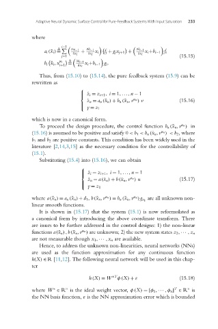
Thus, from (15.10)to(15.14), the pure feedback system (15.9)can be
rewritten as
⎧
⎪ ˙ z i = z i+1 , i = 1,...,n − 1
⎨
α n
˙ z n = a n (¯ x n ) + b n (¯ x n ,v ) v (15.16)
⎪
⎩
y = z 1
which is now in a canonical form.
To proceed the design procedure, the control function b n (¯ x n ,v ) in
α n
(15.16) is assumed to be positive and satisfy 0 < b 1 < b n (¯ x n ,v ) < b 2,where
α n
b 1 and b 2 are positive constants. This condition has been widely used in the
literature [2,14,3,15] as the necessary condition for the controllability of
(15.1).
Substituting (15.4)into(15.16), we can obtain

⎧
⎪ ˙ z i = z i+1 , i = 1,...,n − 1
⎨
α n
˙ z n = a(¯ x n ) + b(¯ x n ,v ) u (15.17)
⎪
⎩
y = z 1
α n α n are all unknown non-
where a(¯ x n ) = a n (¯ x n ) +d 1, b(¯ x n ,v ) = b n (¯ x n ,v )g u ξ
linear smooth functions.
It is shown in (15.17) that the system (15.1) is now reformulated as
a canonical form by introducing the above coordinate transform. There
are issues to be further addressed in the control designs: 1) the non-linear
α n
functions a(¯ x n ),b(¯ x n ,v ) are unknown; 2) the new system states z 2 ,··· ,z n
are not measurable though x 1 ,··· ,x n are available.
Hence, to address the unknown non-linearities, neural networks (NNs)
are used as the function approximation for any continuous function
h(X) ∈ R[11,12]. The following neural network will be used in this chap-
ter

h(X) = W ∗T φ (X) + ε (15.18)

T
n
n
where W ∈ R is the ideal weight vector, φ (X) =[φ 1 ,··· ,φ n ] ∈ R is
∗
the NN basis function, ε is the NN approximation error which is bounded