Page 24 - Adaptive Identification and Control of Uncertain Systems with Nonsmooth Dynamics

Friction Dynamics and Modeling 15

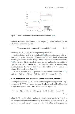
Figure 1.1 Profile of continuously differentiable friction model (1.13).

model is reported, where the friction torque T f can be presented as the
following parameterized form

T f = α 1 [tanh(β 1 ˙x) − tanh(β 2 ˙x)]+ α 2 tanh(β 3 ˙x) + α 3 ˙x, (1.13)

where α 1, α 2, α 3, β 1, β 2, β 3 are all positive parameters.
Unlike of other friction models, Eq. (1.13) has a continuously differen-
tiable property due to the use of function tanh(·), and thus it allows more
flexibility in adaptive control designs. Moreover, as shown in friction model
(1.13), the static friction coefficients are α 1, α 2, and the Stribeck effect is
captured by tanh(β 1 ˙x) − tanh(β 2 ˙x). The Coulomb friction is dominated by
α 2 tanh(β 3 ˙x) and the viscous dissipation is denoted by α 3 ˙x. For further de-
tails on this model, we refer to [6].
As for an example, Fig. 1.1 provides theprofileoffrictionmodel (1.13)
with α 1 = 0.25,α 2 = 0.5,α 3 = 0.01, β 1 = 100, β 2 = 1, and β 3 = 100.

1.2.4 Discontinuous Piecewise Parametric Friction Model

In our previous work [7], a new discontinuous piecewise parametric rep-
resentation (DPPR) of friction has been developed and validated based on
manipulator systems. The DPPR friction model is given by

T f = d 0 + N d r ρ r (0, ˙x − α r (˙x),β r (˙x) − α r (˙x)) + h 1 (˙x) + d N+1h 2 (˙x)
r=1
(1.14)
where ˙x, T f are the velocity and the friction force, respectively. N(≥ 2) is
the number of subintervals obtained by partitioning the domain of ˙x. α r , β r
are the lower and upper boundaries of the r-th subinterval, respectively.