Page 290 - Adsorption, Ion Exchange & Catalysis- 2007, Elsevier - Copy

Else_AIEC-INGLE_cH004.qxd 7/1/2006 6:53 PM Page 286
286 4. Adsorption and Ion Exchange

the corresponding kinetic parameter assuming that the swelling of the resin beads is ne , g-
ligible.

Solution
The first step is to use the kinetic data to eersion of the resin phase ( v aluate the con v X B ):

q t
X B
q max

where q max = 388 mg Pb/g of dry resin and q is gi en by v
t
V L
q ( C o C ) t
t
m
where C is the solution concentration of Pb 2 , V L the solution v and olume, m the resin
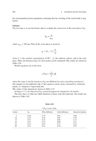
mass. Then, the function f ( X B ) for each model can be estimated. The results are shown in
Table 4.18.
Model equations are in the form

t
fX ( B ) S C t d A ∫
0

where the slope S and the function f ( X B ) are different for each controlling mechanism.
The integral on the righthand side of this equation can be easily estimated by arithmetic
means, i.e. Simpson’ s trapezoidal rule.
able 4.19. The values of this integral are shoT wn in
In Figure 4.17, the function f ( X B ) is plotted against the integral for all models.
The next step is to find out which function is linear with zero intercept. The results are
shown in Table 4.20.

Table 4.18

f(X B ) versus t data
t (min) X B Film diffusion Solid diffusion Reaction kinetics
5 0.18 0.18 0.01 0.06
10 0.26 0.26 0.03 0.10
15 0.34 0.34 0.05 0.13
25 0.43 0.43 0.08 0.17
45 0.54 0.54 0.13 0.23
60 0.61 0.61 0.18 0.27