Page 53 - Advanced_Engineering_Mathematics o'neil

1.5 Additional Applications 33

Of course, this limit is irrelevant in this setting, since the block reaches the bottom in about 5.8
seconds. However, if the ramp is long enough, the block will approach arbitrarily close to 24 feet
per second in velocity. For practical purposes on a sufficiently long ramp, the block will appear
to settle into a constant velocity slide. This is similar to the terminal velocity experienced by an
object falling in a retarding medium.

Electrical Circuits An RLC circuit is one having only constant resistors, capacitors, and induc-
tors (assumed constant here) as elements and an electromotive driving force E(t). The current
i(t) and charge q(t) are related by i(t) = q (t). The voltage drop across a resistor having resis-

tance R is iR, the drop across a capacitor having capacitance C is q/C, and the drop across an
inductor having inductance L is Li .

We can construct differential equations for circuits by using Kirchhoff’s current and voltage
laws. The current law states that the algebraic sum of the currents at any junction of a circuit is
zero. This means that the total current entering the junction must balance the current leaving it
(conservation of energy). The voltage law states that the algebraic sum of the potential rises and
drops around any closed loop in a circuit is zero.
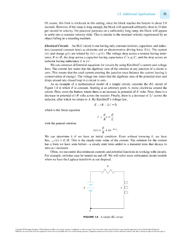
As an example of a mathematical model of a simple circuit, consider the RL circuit of
Figure 1.8 in which E is constant. Starting at an arbitrary point A, move clockwise around the
circuit. First, cross the battery where there is an increase in potential of E volts. Next, there is a

decrease in potential of iR volts across the resistor. Finally, there is a decrease of Li across the
inductor, after which we return to A. By Kirchhoff’s voltage law,
E − iR − Li = 0,

which is the linear equation
E E

i + i =
R L
with the general solution
E
i(t) = + ke −Rt/L .
R
We can determine k if we have an initial condition. Even without knowing k,wehave
lim t→∞ i(t) = E/R. This is the steady-state value of the current. The solution for the current
has a form we have seen before—a steady-state term added to a transient term that decays to
zero as t increases.
Often, we encounter discontinuous currents and potential functions in working with circuits.
For example, switches may be turned on and off. We will solve more substantial circuit models
when we have the Laplace transform at our disposal.
R

E L

A
FIGURE 1.8 A simple RL circuit.

Copyright 2010 Cengage Learning. All Rights Reserved. May not be copied, scanned, or duplicated, in whole or in part. Due to electronic rights, some third party content may be suppressed from the eBook and/or eChapter(s).
Editorial review has deemed that any suppressed content does not materially affect the overall learning experience. Cengage Learning reserves the right to remove additional content at any time if subsequent rights restrictions require it.

October 14, 2010 14:9 THM/NEIL Page-33 27410_01_ch01_p01-42