Page 643 - Advanced_Engineering_Mathematics o'neil

17.2 The Heat Equation on [0, L] 623

0.5
0.5
0.4
0.4
0.3
0.3

0.2
0.2

0.1
0.1

0 0
0 0.5 1 1.5 2 2.5 3 0 0.5 1 1.5 2 2.5 3
x x

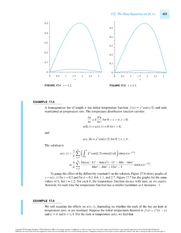
FIGURE 17.4 t = 1.2. FIGURE 17.5 t = 1.3.

EXAMPLE 17.5
2
A homogeneous bar of length π has initial temperature function f (x) = x cos(x/2) and ends
maintained at temperature zero. The temperature distribution function satisfies
2
∂u ∂ u
= k for 0 < x <π,t > 0,
∂t ∂x 2
u(0,t) = u(π,t) = 0for t > 0,
and
2
u(x,0) = x cos(x/2) for 0 ≤ x ≤ π.
The solution is
2 π 2
∞
2
u(x,t) = ξ cos(ξ/2)sin(nξ)dξ sin(nx)e −n kt
π
n=1 0
3
n
∞
n
4 16πn(−1) − 64πn (−1) − 48n − 64n 3 2
= sin(nx)e −n kt .
2
4
6
π 64n − 48n + 12n − 1
n=1
To gauge the effect of the diffusivity constant k on the solution, Figure 17.6 shows graphs of
y = u(x,t) for t = 0.2 and for k = 0.3,0.6, 1.1, and 2.7. Figure 17.7 has the graphs for the same
values of k,but t = 1.2. For each k, the temperature function decays with time, as we expect.
However, for each time the temperature function has a smaller maximum as k increases.
EXAMPLE 17.6
We will examine the effects on u(x,t), depending on whether the ends of the bar are kept at
2
temperature zero, or are insulated. Suppose the initial temperature function is f (x) = x (π − x)
and L = π and k = 1/4. For the ends at temperature zero, we find that

Copyright 2010 Cengage Learning. All Rights Reserved. May not be copied, scanned, or duplicated, in whole or in part. Due to electronic rights, some third party content may be suppressed from the eBook and/or eChapter(s).
Editorial review has deemed that any suppressed content does not materially affect the overall learning experience. Cengage Learning reserves the right to remove additional content at any time if subsequent rights restrictions require it.

October 14, 2010 15:25 THM/NEIL Page-623 27410_17_ch17_p611-640