Page 802 - Advanced_Engineering_Mathematics o'neil

782 CHAPTER 23 Conformal Mappings and Applications

Along a streamline ψ(x, y) = c,
∂ψ ∂ψ
dψ = dx + dy =−v dx + udy = 0,
∂x ∂y
so the normal to the velocity vector is orthogonal to the streamline. This means that the velocity
is tangent to the streamline and justifies the interpretation that the particle of fluid at (x, y) is
moving in the direction of the streamline at this point. We therefore interpret streamlines as the
trajectories of the particles in the fluid. For this reason, graphs of the streamlines form a picture
of the motion of the fluid.

EXAMPLE 23.20
iθ
Let f (z) =−Ke z with K as a positive constant and θ is fixed with 0 ≤ θ ≤ 2π. Write
f (z) =−K(cos(θ) + i sin(θ))(x + iy)
=−K(x cos(θ) − y sin(θ)) − iK(y cos(θ) + x sin(θ)).
If f (z) = ϕ(x, y) + iψ(x, y), then
ϕ(x, y) =−K(x cos(θ) − y sin(θ))
and
ψ(x, y) =−K(y cos(θ) + x sin(θ)).
Since K is constant, equipotential curves are graphs of
x cos(θ) − y sin(θ) = k
or
y = cot(θ) + b
in which b = k sec(θ) is constant. These are straight lines with slope cot(θ).
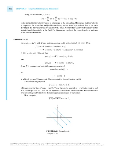
Streamlines are graphs of
ψ(x, y) =−tan(θ)x + d,
which are straight lines of slope −tan(θ). These lines make an angle π − θ with the positive real
axis, as in Figure 23.33. These are the trajectories of the flow. The streamlines and equipotential
lines are orthogonal with slopes that are negative reciprocals of each other.
Now compute
f (z) = −Ke =−Ke −iθ ,
iθ

z

θ

FIGURE 23.33 Streamlines in
Example 23.20.

Copyright 2010 Cengage Learning. All Rights Reserved. May not be copied, scanned, or duplicated, in whole or in part. Due to electronic rights, some third party content may be suppressed from the eBook and/or eChapter(s).
Editorial review has deemed that any suppressed content does not materially affect the overall learning experience. Cengage Learning reserves the right to remove additional content at any time if subsequent rights restrictions require it.

October 14, 2010 15:39 THM/NEIL Page-782 27410_23_ch23_p751-788