Page 803 - Advanced_Engineering_Mathematics o'neil

23.4 Models of Plane Fluid Flow 783

since θ is real. This implies that the velocity has constant magnitude K.Insum, f models a
uniform flow with velocity of a constant magnitude K moving at an angle π −θ with the positive
real axis.

EXAMPLE 23.21
2
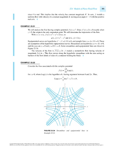
We will analyze the flow having complex potential f (z) = z . Since f (z) = 2z = 0 exactly when

z = 0, the origin is the only stagnation point. We will determine the trajectories of the flow.
2
2
With z = x + iy, f (z) = x − y + 2ixy,so
2
2
ϕ(x, y) = x − y and ψ(x, y) = 2xy.
2
2
Equipotential curves are hyperbolas x − y =k if k =0, and straight lines y =±x if k =0. These
are asymptotes of the hyperbolic equipotential curves. Streamlines are hyperbolas xy =c if c =0,
and the axes are x = 0 and y = 0if c = 0. Some streamlines and equipotential lines are shown in
Figure 23.34.
The velocity of the flow is f (z) = 2z. f models a nonuniform flow having velocity of

magnitude 2|z| at z. This flow moves along the hyperbolic streamlines with the axes acting as
barriers of the flow (think of sides of a container holding the fluid).
EXAMPLE 23.22
Consider the flow associated with the complex potential
iK
f (z) = Log(z),
2π
for z = 0, where Log(z) is the logarithm of z having argument between 0 and 2π. Thus,
1
2
2
Log(z) = ln(x + y ) + iθ,
2
x
2

1

y
−2 −1 0 1 2

−1

−2

FIGURE 23.34 Streamlines and equipotential lines in
Example 23.21.

Copyright 2010 Cengage Learning. All Rights Reserved. May not be copied, scanned, or duplicated, in whole or in part. Due to electronic rights, some third party content may be suppressed from the eBook and/or eChapter(s).
Editorial review has deemed that any suppressed content does not materially affect the overall learning experience. Cengage Learning reserves the right to remove additional content at any time if subsequent rights restrictions require it.

October 14, 2010 15:39 THM/NEIL Page-783 27410_23_ch23_p751-788