Page 226 - Advanced engineering mathematics

206 CHAPTER 7 Matrices and Linear Systems

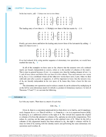
In the last matrix, add −3 times row two to row three:

⎛ ⎞ ⎛ ⎞
0101 1 0101 1
⎜ 0010 0 ⎟ ⎜ 0010 0 ⎟
⎜ ⎟ → ⎜ ⎟ .
⎝ 0030 −4 ⎠ ⎝ 0000 −4 ⎠
0000 0 0000 0
The leading entry of row three is −4. Multiply row three of the last matrix by −1/4:

⎛ ⎞ ⎛ ⎞
0101 1 01011
⎜ 0010 0 ⎟ ⎜ 00100 ⎟
⎜ ⎟ → ⎜ ⎟ .
⎝ 0000 −4 ⎠ ⎝ 00001 ⎠
0000 0 00000
Finally, get zeros above and below the leading entry in row three of the last matrix by adding −1
times row three to row 1:
⎛ ⎞ ⎛ ⎞
01011 01010
00100 00100
⎜ ⎟ ⎜ ⎟
→ = A R .
⎜ ⎟ ⎜ ⎟
⎝ 00001 ⎠ ⎝ 00001 ⎠
00000 00000
If we had reduced A by using another sequence of elementary row operations, we would have
reached the same A R .

In all of the examples we have seen so far, observe that the nonzero rows of a reduced
matrix are linearly independent m-vectors, where m is the number of columns of the matrix.
This is true in general because, if row i is a nonzero row, then the leading element of row i is
1, and all rows above and below this row have 0 in this column. Thus each nonzero row vector
in A R has a 1 in a coordinate where all the other row vectors have zeros. Later, when we deal
with rank and solve systems of equations, it will be important to know that the nonzero rows
of A R are linearly independent in the row space of A, hence they form a basis for this row
space.
The elementary row operations used to reduce a matrix A can be achieved by multiplying A
on the left by some elementary matrix (which is a product of elementary matrices). In view of
Theorems 7.5 and 7.7, we can state the following.

THEOREM 7.8

Let A be any matrix. Then there is a matrix such that
A = A R .

Given A, there is a convenient notational device that allows us to find A R and simultane-
.
.
ously. Suppose A is n ×m. Then will be n ×n. Form the n ×(m +n) augmented matrix [A.I n ]
by putting I n as n additional columns to the right of A. The vertical dots separate the original
m columns of A from the adjoined n columns of I n , and play no role in the computations. Now
reduce A, carrying out the same operations on the adjoined rows of I n . When A (the left m
columns of this augmented matrix) has been reduced to A R , the right n columns will be ,
since we form by starting with the identity matrix and performing the same elementary row
operations used to reduce A.

Copyright 2010 Cengage Learning. All Rights Reserved. May not be copied, scanned, or duplicated, in whole or in part. Due to electronic rights, some third party content may be suppressed from the eBook and/or eChapter(s).
Editorial review has deemed that any suppressed content does not materially affect the overall learning experience. Cengage Learning reserves the right to remove additional content at any time if subsequent rights restrictions require it.

October 14, 2010 14:23 THM/NEIL Page-206 27410_07_ch07_p187-246