Page 222 - Advanced engineering mathematics

202 CHAPTER 7 Matrices and Linear Systems

⎛ ⎞ ⎛ ⎞
0 −3 1 0 −3 1
O 3 O 4
−→ 2 1 0 ⎠ −→ −8 −4 0 ⎠ = .
⎝
⎝
1 0 0 1 0 0
Then
⎛ ⎞⎛ ⎞
0 −3 1 0 −1 1 4
A = −8 −4 0 ⎠⎝ 9 3 7 −7 ⎠
⎝
1 0 0 0 2 1 5
⎛ ⎞
−27 −7 −20 26
= −84 −4 −36 −4 ⎠ = B.
⎝
6 −1 1 4
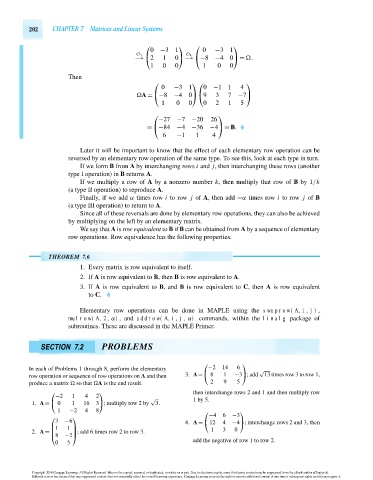
Later it will be important to know that the effect of each elementary row operation can be
reversed by an elementary row operation of the same type. To see this, look at each type in turn.
If we form B from A by interchanging rows i and j, then interchanging these rows (another
type I operation) in B returns A.
If we multiply a row of A by a nonzero number k, then multiply that row of B by 1/k
(a type II operation) to reproduce A.
Finally, if we add α times row i to row j of A, then add −α times row i to row j of B
(a type III operation) to return to A.
Since all of these reversals are done by elementary row operations, they can also be achieved
by multiplying on the left by an elementary matrix.
We say that A is row equivalent to B if B can be obtained from A by a sequence of elementary
row operations. Row equivalence has the following properties.

THEOREM 7.6
1. Every matrix is row equivalent to itself.
2. If A is row equivalent to B, then B is row equivalent to A.
3. If A is row equivalent to B, and B is row equivalent to C, then A is row equivalent
to C.

Elementary row operations can be done in MAPLE using the swaprow(A,i,j),
mulrow(A,2,α), and addrow(A,i,j,α) commands, within the linalg package of
subroutines. These are discussed in the MAPLE Primer.

SECTION 7.2 PROBLEMS

⎛ ⎞
In each of Problems 1 through 8, perform the elementary −2 14 6 √
row operation or sequence of row operations on A and then 3. A= ⎝ 8 1 −3 ⎠ ;add 13 times row 3 to row 1,
produce a matrix so that A is the end result. 2 9 5
then interchange rows 2 and 1 and then multiply row
⎛ ⎞
−2 1 4 2
√ 1by5.
1. A = ⎝ 0 1 16 3 ⎠ ; multiply row 2 by 3.
1 −2 4 8 ⎛ ⎞
−4 6 −3
⎛ ⎞
3 −6 4. A = ⎝ 12 4 −4 ⎠ ; interchange rows 2 and 3, then
1 1
⎜ ⎟ 1 3 0
2. A = ⎜ ⎟ ; add 6 times row 2 to row 3.
⎝ 8
−2 ⎠
add the negative of row 1 to row 2.
0 5
Copyright 2010 Cengage Learning. All Rights Reserved. May not be copied, scanned, or duplicated, in whole or in part. Due to electronic rights, some third party content may be suppressed from the eBook and/or eChapter(s).
Editorial review has deemed that any suppressed content does not materially affect the overall learning experience. Cengage Learning reserves the right to remove additional content at any time if subsequent rights restrictions require it.
October 14, 2010 14:23 THM/NEIL Page-202 27410_07_ch07_p187-246