Page 428 - Advanced engineering mathematics

408 CHAPTER 12 Vector Integral Calculus

12.9 Stokes’s Theorem

In Section 12.7, we suggested a lifting of Green’s theorem to three dimensions to arrive at
Stokes’s theorem. That discussion passed quickly over some subtleties which we will now
address more carefully.
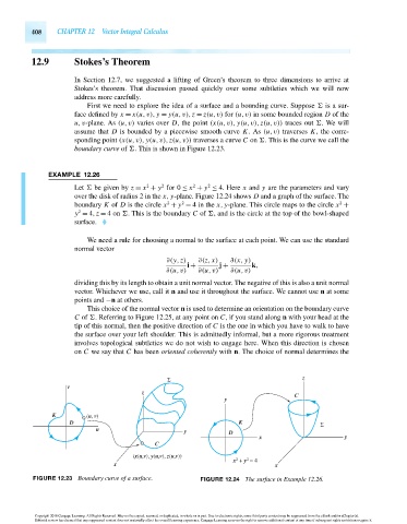
First we need to explore the idea of a surface and a bounding curve. Suppose is a sur-
face defined by x = x(u,v), y = y(u,v), z = z(u,v) for (u,v) in some bounded region D of the
u,v-plane. As (u,v) varies over D, the point (x(u,v), y(u,v), z(u,v)) traces out . We will
assume that D is bounded by a piecewise smooth curve K.As (u,v) traverses K, the corre-
sponding point (x(u,v), y(u,v), z(u,v)) traverses a curve C on . This is the curve we call the
boundary curve of . This is shown in Figure 12.23.

EXAMPLE 12.26
2
2
2
2
Let be given by z = x + y for 0 ≤ x + y ≤ 4. Here x and y are the parameters and vary
over the disk of radius 2 in the x, y-plane. Figure 12.24 shows D and a graph of the surface. The
2 2 2
boundary K of D is the circle x + y = 4inthe x, y-plane. This circle maps to the circle x +
2
y = 4, z = 4on . This is the boundary C of , and is the circle at the top of the bowl-shaped
surface.
We need a rule for choosing a normal to the surface at each point. We can use the standard
normal vector
∂(y, z) ∂(z, x) ∂(x, y)
i + j + k,
∂(u,v) ∂(u,v) ∂(u,v)
dividing this by its length to obtain a unit normal vector. The negative of this is also a unit normal
vector. Whichever we use, call it n and use it throughout the surface. We cannot use n at some
points and −n at others.
This choice of the normal vector n is used to determine an orientation on the boundary curve
C of . Referring to Figure 12.25, at any point on C, if you stand along n with your head at the
tip of this normal, then the positive direction of C is the one in which you have to walk to have
the surface over your left shoulder. This is admittedly informal, but a more rigorous treatment
involves topological subtleties we do not wish to engage here. When this direction is chosen
on C we say that C has been oriented coherently with n. The choice of normal determines the

Σ z
v
z C
y

K (u, v)
D K Σ
u y D
x y
C
(x(u,v), y(u,v), z(u,v))
2
2
x + y = 4
x x
FIGURE 12.23 Boundary curve of a surface. FIGURE 12.24 The surface in Example 12.26.

Copyright 2010 Cengage Learning. All Rights Reserved. May not be copied, scanned, or duplicated, in whole or in part. Due to electronic rights, some third party content may be suppressed from the eBook and/or eChapter(s).
Editorial review has deemed that any suppressed content does not materially affect the overall learning experience. Cengage Learning reserves the right to remove additional content at any time if subsequent rights restrictions require it.

October 14, 2010 14:53 THM/NEIL Page-408 27410_12_ch12_p367-424