Page 429 - Advanced engineering mathematics

12.9 Stokes’s Theorem 409

z
(0, 0, 3)
C: boundary curve

Σ
z
N(3, 0, 3)
Σ

n
C
y
y

x
x
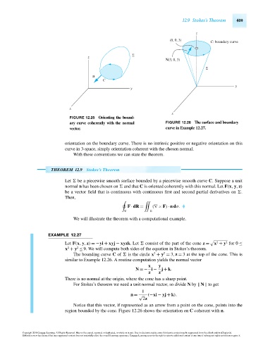
FIGURE 12.25 Orienting the bound-
ary curve coherently with the normal FIGURE 12.26 The surface and boundary
vector. curve in Example 12.27.

orientation on the boundary curve. There is no intrinsic positive or negative orientation on this
curve in 3-space, simply orientation coherent with the chosen normal.
With these conventions we can state the theorem.

THEOREM 12.9 Stokes’s Theorem

Let be a piecewise smooth surface bounded by a piecewise smooth curve C. Suppose a unit
normal n has been chosen on and that C is oriented coherently with this normal. Let F(x, y, z)
be a vector field that is continuous with continuous first and second partial derivatives on .
Then,

F · dR = (∇× F) · ndσ.
C
We will illustrate the theorem with a computational example.

EXAMPLE 12.27

2
2
Let F(x, y, z) =−yi + xyj − xyzk.Let consist of the part of the cone z = x + y for 0 ≤
2
2
x + y ≤ 9. We will compute both sides of the equation in Stokes’s theorem.
2
2
The bounding curve C of is the circle x + y = 3, z = 3 at the top of the cone. This is
similar to Example 12.26. A routine computation yields the normal vector
x y
N =− i − j + k.
z z
There is no normal at the origin, where the cone has a sharp point.
For Stokes’s theorem we need a unit normal vector, so divide N by N to get
1
n = √ (−xi − yj + k).
2z
Notice that this vector, if represented as an arrow from a point on the cone, points into the
region bounded by the cone. Figure 12.26 shows the orientation on C coherent with n.

Copyright 2010 Cengage Learning. All Rights Reserved. May not be copied, scanned, or duplicated, in whole or in part. Due to electronic rights, some third party content may be suppressed from the eBook and/or eChapter(s).
Editorial review has deemed that any suppressed content does not materially affect the overall learning experience. Cengage Learning reserves the right to remove additional content at any time if subsequent rights restrictions require it.

October 14, 2010 14:53 THM/NEIL Page-409 27410_12_ch12_p367-424