Page 477 - Advanced engineering mathematics

13.6 Complex Fourier Series 457

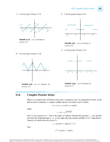
9. f has the graph of Figure 13.19. 11. f has the graph of Figure 13.21.

y
y
1
2
x
–3 –2 –1 1 2 3
1
–1
x
–3 –1 1 3

FIGURE 13.19 f (x) in Problem 9,
Section 13.5.
FIGURE 13.21 f (x) in Problem 11,
Section 13.5.

12. f has the graph of Figure 13.22.

10. f has the graph of Figure 13.20. y

y
k
k

x x
–2 2 4 –2 –1 0 1 2 3

FIGURE 13.20 f (x) in Problem 10, FIGURE 13.22 f (x) in Problem 12,
Section 13.5. Section 13.5.

13.6 Complex Fourier Series

There is a complex form of Fourier series that is sometimes used. As preparation for this, recall
that, in polar coordinates, a complex number (point in the plane) can be written
z = x + iy =r cos(θ) + ir sin(θ)
where

2
r =|z|= x + y 2
and θ is an argument of z. This is the angle (in radians) between the positive x− axis and the
line from the origin through (x, y), or this angle plus any integer multiple of 2π. Using Euler’s
formula, we obtain the polar form of z:
iθ
z =r[cos(θ) + i sin(θ)]=re .
Now
iθ
e = cos(θ) + i sin(θ),

Copyright 2010 Cengage Learning. All Rights Reserved. May not be copied, scanned, or duplicated, in whole or in part. Due to electronic rights, some third party content may be suppressed from the eBook and/or eChapter(s).
Editorial review has deemed that any suppressed content does not materially affect the overall learning experience. Cengage Learning reserves the right to remove additional content at any time if subsequent rights restrictions require it.

October 14, 2010 14:57 THM/NEIL Page-457 27410_13_ch13_p425-464