Page 483 - Advanced engineering mathematics

13.7 Filtering of Signals 463

1 1

0.5
0.5
0 –3 –2 –1 0 1 2 3
–3 –2 –1 0 1 2 3 0

–0.5
–0.5

–1
–1

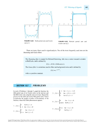
FIGURE 13.24 Tenth partial sum and Cesàro
FIGURE 13.25 Thirtieth partial sum and
sum of f .
Cesàro sum of f .

There are many filters used in signal analysis. Two of the more frequently used ones are the
Hamming and Gauss filters.

The Hamming filter is named for Richard Hamming, who was a senior research scientist
at Bell Labs, and is defined by
Z(t) = 0.54 + 0.46cos(πt).
The Gauss filter is sometimes used to filter out background noise and is defined by
2 2
Z(t) = e −απ t ,
with α a positive constant.

SECTION 13.7 PROBLEMS

⎧
In each of Problems 1 through 5, graph the function, the ⎪−1 for −1 ≤ t < −1/2
⎨
fifth partial sum of its Fourier series on the interval, and 3. f (t) = 0 for −1/2 ≤ t < 1/2
the fifth Cesàro sum, using the same set of axes. Repeat this ⎪
1 for 1/2 ≤ t < 1
⎩
process for the tenth and twenty-fifth partial sums. Notice
in particular the graphs at points of discontinuity of the

function, where the Gibbs phenomenon appears. 0 for −3 ≤ t < 0
4. f (t) =
cos(t) for 0 ≤ t < 3

1 for 0 ≤ t < 2
1. f (t) =
−1for −2 ≤ t < 0
2 + t for −1 ≤ t < 0
5. f (t) =

t 2 for −2 ≤ t < 1 7 for 0 ≤ t < 1
2. f (t) =
2 + t for 1 ≤ t < 2
Copyright 2010 Cengage Learning. All Rights Reserved. May not be copied, scanned, or duplicated, in whole or in part. Due to electronic rights, some third party content may be suppressed from the eBook and/or eChapter(s).
Editorial review has deemed that any suppressed content does not materially affect the overall learning experience. Cengage Learning reserves the right to remove additional content at any time if subsequent rights restrictions require it.
October 14, 2010 14:57 THM/NEIL Page-463 27410_13_ch13_p425-464