Page 494 - Advanced engineering mathematics

474 CHAPTER 14 The Fourier Integral and Transforms

As an illustration, we will compute the inverse of this Fourier transform. By equation
(14.11),
1 ∞
−1 ˆ ˆ iωt
F [ f ](t) = f (ω)e dω
2π
−∞
1 ∞ 1 − cos(ω)
iωt
= e dω
π ω 2
−∞
= π(t + 1)sgn(t + 1) + π(t − 1)sgn(t − 1) − 2sgn(t).
This integration was done using MAPLE, in which

⎧
⎪1 for t > 0
⎨
sgn(t) = −1 for t < 0
⎪
0 for t = 0.
⎩
−1 ˆ
By considering cases t <−1, −1<t <1 and t >1, it is routine to verify that indeed F [ f ](t)=
f (t) in this example.

In the context of the Fourier transform, the amplitude spectrum of a signal f (t) is the graph
ˆ
of | f (ω)|.

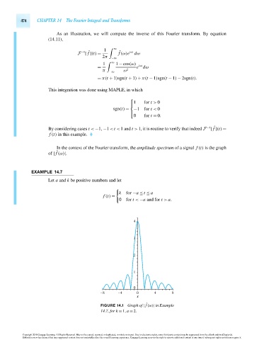
EXAMPLE 14.7

Let a and k be positive numbers and let

k for −a ≤ t ≤ a
f (t) =
0 for t < −a and for t > a.

4

3

2

1

0
–8 –4 0 4 8
x
FIGURE 14.1 Graph of | ˆ f (ω)| in Example
14.7, for k = 1,a = 2.

Copyright 2010 Cengage Learning. All Rights Reserved. May not be copied, scanned, or duplicated, in whole or in part. Due to electronic rights, some third party content may be suppressed from the eBook and/or eChapter(s).
Editorial review has deemed that any suppressed content does not materially affect the overall learning experience. Cengage Learning reserves the right to remove additional content at any time if subsequent rights restrictions require it.

October 14, 2010 16:43 THM/NEIL Page-474 27410_14_ch14_p465-504