Page 495 - Advanced engineering mathematics

14.3 The Fourier Transform 475

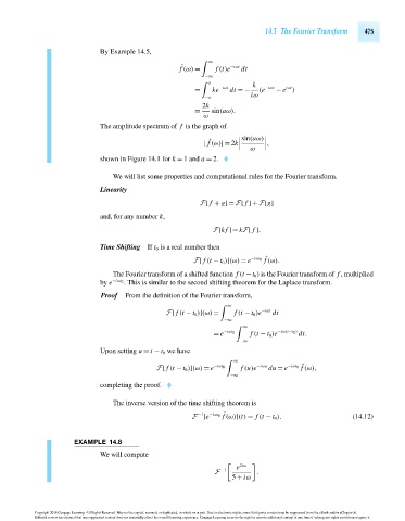
By Example 14.5,
∞

ˆ −iωt
f (ω) = f (t)e dt
−∞
a k
iωt
= ke −iωt dt =− (e −iωt − e )
−a iω
2k
= sin(aω).
ω
The amplitude spectrum of f is the graph of

ˆ sin(aω) ,
| f (ω)|= 2k
ω
shown in Figure 14.1 for k = 1 and a = 2.
We will list some properties and computational rules for the Fourier transform.
Linearity

F[ f + g]= F[ f ]+ F[g]
and, for any number k,
F[kf ]= kF[ f ].

Time Shifting If t 0 is a real number then

F[ f (t − t 0 )](ω) = e −iωt 0 ˆ
f (ω).
The Fourier transform of a shifted function f (t −t 0 ) is the Fourier transform of f , multiplied
by e −iωt 0 . This is similar to the second shifting theorem for the Laplace transform.

Proof From the definition of the Fourier transform,
∞

F[ f (t − t 0 )](ω) = f (t − t 0 )e −iωt dt
−∞

∞
= e −iωt 0 f (t − t 0 )e −iω(t−t 0 ) dt.
−∞
Upon setting u = t − t 0 we have

∞
F[ f (t − t 0 )](ω) = e −iωt 0 f (u)e −iωu du = e −iωt 0 ˆ
f (ω),
−∞
completing the proof.
The inverse version of the time shifting theorem is
−1
F [e −iωt 0 ˆ (14.12)
f (ω)](t) = f (t − t 0 ).
EXAMPLE 14.8

We will compute
2iω
e
−1
F .
5 + iω

Copyright 2010 Cengage Learning. All Rights Reserved. May not be copied, scanned, or duplicated, in whole or in part. Due to electronic rights, some third party content may be suppressed from the eBook and/or eChapter(s).
Editorial review has deemed that any suppressed content does not materially affect the overall learning experience. Cengage Learning reserves the right to remove additional content at any time if subsequent rights restrictions require it.

October 14, 2010 16:43 THM/NEIL Page-475 27410_14_ch14_p465-504