Page 507 - Advanced engineering mathematics

14.3 The Fourier Transform 487

14.3.4 Low-Pass and Bandpass Filters
If f is a signal with finite energy, then the spectrum of f is given by its Fourier transform. If
ω 0 is a positive number and f is not band-limited, we can replace f with a band-limited signal
having bandwidth not exceeding ω 0 by applying a low-pass filter which cuts f (ω) off at
ˆ
f ω 0
frequencies outside the range [−ω 0 ,ω 0 ]. That is, let

ˆ
f (ω) for −ω 0 ≤ ω ≤ ω 0 ,
ˆ
f ω 0 (ω) =
0 for |ω| >ω 0 .
ˆ
This defined the transform f ω 0 , from which we recover f ω 0 by the inverse Fourier transform
1 ∞ 1 ω 0
(t) = ˆ ω)e iωt dω = ˆ (ω)e iωt dω.
f ω 0 f ω 0 f ω 0
2π 2π
−∞ −ω 0
Applying a low-pass filter is actually a windowing process. Define the characteristic function χ I
of an interval I by

1 for t in I,
χ I (t) =
0 for t not in I.
Then

ˆ ˆ
f ω 0 (ω) = χ [−ω 0 ,ω 0 ] (ω) f (ω) (14.15)
ˆ
so we have windowed f (ω) with the characteristic function χ [−ω 0 ,ω 0 ] . More succinctly,
ˆ = χ [−ω 0 ,ω 0 ] f .
ˆ
f ω 0
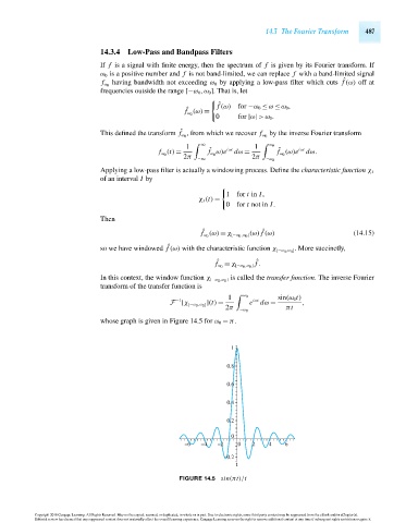
In this context, the window function χ [−ω 0 ,ω 0 ] is called the transfer function. The inverse Fourier
transform of the transfer function is
1 ω 0 sin(ω 0 t)
−1 iωt
F [χ [−ω 0 ,ω 0 ] ](t) = e dω = ,
2π −ω 0 πt
whose graph is given in Figure 14.5 for ω 0 = π.

1

0.8

0.6

0.4

0.2

0
–6 –4 –2 0 2 4 6
–0.2
t
FIGURE 14.5 sin(πt)/t

Copyright 2010 Cengage Learning. All Rights Reserved. May not be copied, scanned, or duplicated, in whole or in part. Due to electronic rights, some third party content may be suppressed from the eBook and/or eChapter(s).
Editorial review has deemed that any suppressed content does not materially affect the overall learning experience. Cengage Learning reserves the right to remove additional content at any time if subsequent rights restrictions require it.

October 14, 2010 16:43 THM/NEIL Page-487 27410_14_ch14_p465-504