Page 508 - Advanced engineering mathematics

488 CHAPTER 14 The Fourier Integral and Transforms

Now recall time and frequency convolution for the Fourier transform. Analog filtering in the
time variable is done by convolution. If ϕ(t) is the filter function, then the effect of filtering f
by ϕ is
∞

f ϕ (t) = (ϕ ∗ f )(t) = ϕ(τ) f (t − τ)dτ.
−∞
Take the Fourier transform of this equation to obtain
ˆ
f ϕ (ω) =ˆϕ(ω) f (ω).
ˆ
We therefore filter f in the frequency variable by taking a product of the Fourier transform of
the filter function ϕ with the transform of f .
Using the convolution theorem, we can formulate equation (14.15) as

sin(ω 0 t)
(t) = ∗ f (t) .
f ω 0
πt
This gives the low-pass filtering of f as the convolution of the Shannon sampling function
with f .
from f . This filters out frequen-
In low-pass filtering, we produce a band-limited signal f ω 0
cies outside of [−ω 0 ,ω 0 ]. In a similar kind of filtering, called bandpass filtering, we want to filter
out the effects of the signal outside of given bandwidths. A band-limited signal f can always be
decomposed into a sum of signals, each of which carries the information content of f within a
specified frequency band. To see how to do this suppose f is band-limited with bandwidth
.
Consider a finite increasing sequence of frequencies

0 <ω 1 <ω 2 < ··· <ω N =
.
For j = 1,2,··· , N, define a bandwidth filter function β j by means of its transfer function:
ˆ β j = χ [−ω j ,−ω j−1 ] + χ [ω j−1 ,ω j ] .

This is a sum of characteristic functions of frequency intervals, and is zero outside of these
intervals and 1 for −ω j ≤ ω ≤−ω j−1 and ω j−1 ≤ ω ≤ ω j . The bandwidth filter function β j (t),
which filters the frequency content of f (t) outside of the frequency range [ω j−1 ,ω j ], is obtained
as the inverse Fourier transform of ˆ β j (ω). We obtain
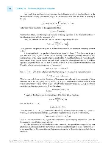
sin(ω j t) − sin(ω j−1 t)
β j (t) = .
πt
A graph of this function is shown in Figure 14.6. Now define functions
sin(ω 0 t)
f 0 (t) = ∗ f (t)
πt
and, for j = 1,2,··· , N,
f j (t) = β j (t) ∗ f (t).

Then, for j =1,2,··· , N, f j (t) carries the content of f (t) in the frequency range ω j−1 ≤ω ≤ω j ,
while f 0 (t) carries the content in [0,ω 0 ], the low-frequency range of f (t). Furthermore,
f (t) = f 0 (t) + f 1 (t) + ··· + f N (t).
This is a decomposition of the signal into components, each carrying information about the
frequency in a specific frequency interval.
We conclude this section with an observation connecting low-pass filters to a previously seen
phenomenon. In signal analysis, the Gibbs phenomenon can be thought of as the step response of
a low-pass filter. In this context the oscillations near the point of discontinuity are called ringing
artifacts.

Copyright 2010 Cengage Learning. All Rights Reserved. May not be copied, scanned, or duplicated, in whole or in part. Due to electronic rights, some third party content may be suppressed from the eBook and/or eChapter(s).
Editorial review has deemed that any suppressed content does not materially affect the overall learning experience. Cengage Learning reserves the right to remove additional content at any time if subsequent rights restrictions require it.

October 14, 2010 16:43 THM/NEIL Page-488 27410_14_ch14_p465-504