Page 179 - Aerodynamics for Engineering Students

162 Aerodynamics for Engineering Students

V1=V*=O Vl =V2# 0

Fig. 4.2

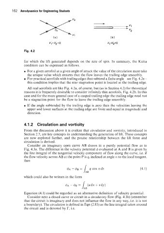
for which the lift generated depends on the rate of spin. In summary, the Kutta
condition can be expressed as follows.
0 For a given aerofoil at a given angle of attack the value of the circulation must take
the unique value which ensures that the flow leaves the trailing edge smoothly.
For practical aerofoils with trailing edges that subtend a finite angle see Fig. 4.2a -
~
this condition implies that the rear stagnation point is located at the trailing edge.
All real aerofoils are like Fig. 4.2a, of course, but (as in Section 4.2) for theoretical
reasons it is frequently desirable to consider infinitely thin aerofoils, Fig. 4.2b. In this
case and for the more general case of a cusped trailing edge the trailing edge need not
be a stagnation point for the flow to leave the trailing edge smoothly.
0 If the angle subtended by the trailing edge is zero then the velocities leaving the
upper and lower surfaces at the trailing edge are finite and equal in magnitude and
direction.

4.1.2 Circulation and vorticity

From the discussion above it is evident that circulation and vorticity, introduced in
Section 2.7, are key concepts in understanding the generation of lift. These concepts
are now explored further, and the precise relationship between the lift force and
circulation is derived.
Consider an imaginary open curve AB drawn in a purely potential flow as in
Fig. 4.3a. The difference in the velocity potential 4 evaluated at A and B is given by
the line integral of the tangential velocity component of flow along the curve, i.e. if
the flow velocity across AB at the point P is q, inclined at angle a to the local tangent,
then

which could also be written in the form
s,,
$A-~B= (Udx+vdy)

Equation (4.1) could be regarded as an alternative definition of velocity potential.
Consider next a closed curve or circuit in a circulatory flow (Fig. 4.3b) (remember
that the circuit is imaginary and does not influence the flow in any way, Le. it is not
a boundary). The circulation is defined in Eqn (2.83) as the line integral taken around
the circuit and is denoted by I?, i.e.