Page 188 - Aerodynamics for Engineering Students

Two-dimensional wing theory 171

Fig. 4.9

thin. He was thereby able to determine the aerofoil shape required for specified
aerofoil characteristics. This made the theory a practical tool for aerodynamic
design. However, as remarked above, the use of conformal transformation is
restricted to two dimensions. Fortunately, it is not necessary to use Glauert’s
approach to obtain his final results. In Section 4.3, later developments are followed
using a method that does not depend on conformal transformation in any way and,
accordingly, in principle at least, can be extended to three dimensions.
Thin aerofoil theory and its applications are described in Sections 4.3 to 4.9. As the
name suggests the method is restricted to thin aerofoils with small camber at small
angles of attack. This is not a major drawback since most practical wings are fairly
thin. A modern computational method that is not restricted to thin aerofoils is
described in Section 4.10. This is based on the extension of the panel method of
Section 3.5 to lifting flows. It was developed in the late 1950s and early 1960s by Hess
and Smith at Douglas Aircraft Company.

*
v.
4.3 <The general thin aerofoil theory
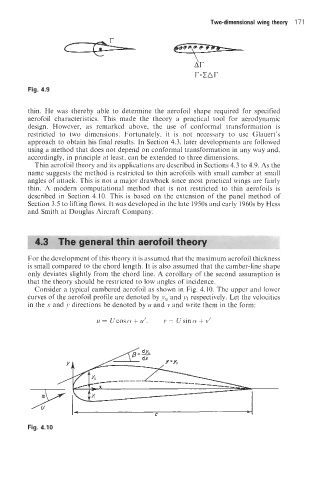
For the development of this theory it is assumed that the maximum aerofoil thickness
is small compared to the chord length. It is also assumed that the camber-line shape
only deviates slightly from the chord line. A corollary of the second assumption is
that the theory should be restricted to low angles of incidence.
Consider a typical cambered aerofoil as shown in Fig. 4.10. The upper and lower
curves of the aerofoil profile are denoted by y, and yl respectively. Let the velocities
in the x and y directions be denoted by u and v and write them in the form:

u= UCOSQ+U’. v= Usincu+v‘

Fig. 4.10