Page 85 - Aerodynamics for Engineering Students

68 Aerodynamics for Engineering Students

Therefore, true air speed = Ma = 0.728 x 340.3
248 m s-' = 89 1 km h-'
In this example, ~7 = 1 and therefore there is no effect due to density, Le. the difference is due
entirely to compressibility. Thus it is seen that neglecting compressibility in the calibration has
led the air-speed indicator to overestimate the true air speed by 59 km h-' .

2,4 Two-dimensional flow

Consider flow in two dimensions only. The flow is the same as that between two planes set
parallel and a little distance apart. The fluid can then flow in any direction between and
parallel to the planes but not at right angles to them. This means that in the subsequent
mathematics there are only two space variables, x and y in Cartesian (or rectangular)
coordinates or r and 0 in polar coordinates. For convenience, a unit length of the flow
field is assumed in the z direction perpendicular to x and y. This simplifies the treatment
of two-dimensional flow problems, but care must be taken in the matter of units.
In practice if two-dimensional flow is to be simulated experimentally, the method
of constraining the flow between two close parallel plates is often used, e.g. small
smoke tunnels and some high-speed tunnels.
To summarize, two-dimensional flow is fluid motion where the velocity at all
points is parallel to a given plane.
We have already seen how the principles of conservation of mass and momentum
can be applied to one-dimensional flows to give the continuity and momentum
equations (see Section 2.2). We will now derive the governing equations for
two-dimensional flow. These are obtained by applying conservation of mass and
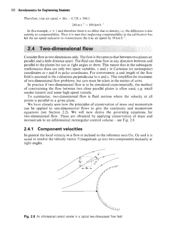
momentum to an infinitesimal rectangular control volume - see Fig. 2.8.

2.4.1 Component velocities
In general the local velocity in a flow is inclined to the reference axes Ox, Oy and it is
usual to resolve the velocity vector ?(magnitude q) into two components mutually at
right-angles.

Fig. 2.8 An infinitesimal control volume in a typical two-dimensional flow field