Page 112 - Algorithm Collections for Digital Signal Processing Applications using MATLAB

100 Chapter 3

5. ORTHONORMAL VECTORS

The vectors a, b, c are defined as the orthogonal vectors if their inner product
matrix is the diagonal matrix. (i.e) dot product of the vector a with itself is
some constant, whereas the dot product of the vector a with b is 0.
If the diagonal matrix obtained is the identity matrix, then the vectors are
called as orthonormal vectors.

5.1 Gram-Schmidt Orthogonalization Procedure

Consider the set of independent vectors v1, v2 and v3 which spans the
particular vector space ‘S’. (i.e) All the vectors in the space ‘S’ are repre-
sented as the linear combination of the independent vectors (v2, v2, v3).
They are called basis.
It is possible to identify the another set of independent vectors o1, o2 and
o3 which spans the space S such that the vectors o1, o2 and o3 are
orthonormal to each other. The steps involved in obtaining the orthornormal
vectors corresponding to the independent vectors are described below.
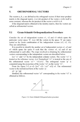
Let ‘v1’ and ‘v2’ be the independent column vectors. The vector ‘v1’ is
treated as the reference vector. (i.e) Normalized ‘v1’ is treated as the one of
the orthonormal vector ‘o1’= ‘v1/||v1||’. The orthogonal vector ‘p’ is
computed using the projection of the vector ‘v2’ on the vector ‘v1’.
T
T
From the figure 3-5 p=v2- [(o1 v2) / (o1 o1)] o1. The orthonormal
vector is the normalized form of the vector ‘p’.
o2 = p / ||p||
Similarly the orthonormal vector ‘o3’ corresponding to the vector ‘v3’ is
obtained as follows.

Figure 3-6. Gram-Schmidt Orthogonalization procedure