Page 67 -

Chapter 2 ■ Edge-Detection Techniques 41

σ+0.8 and σ−0.8 as standard deviation values, does two convolutions, locates
two sets of zero crossings, and merges the resulting edge pixels into a single
image. The result is displayed and is stored in a file named marr.jpg.
Figure 2.11 illustrates the steps in this process, using the chess image (no
noise) as an example. Figures 2.11a and b shows the original image after
being convolved with the LoGs, having σ values of 1.2 and 2.8, respectively.
Figures 2.11c and 2.11d are the responses from these two different values
of σ, and Figure 2.11e shows the result of merging the edge pixels in these
two images.

(a) (b) (c) (d) (e)
Figure 2.11: Steps in the computation of the Marr-Hildreth edge detector. (a) Convolution
of the original image with the LoG having σ = 1.2. (b) Convolution of the image with
the LoG having σ = 2.8. (c) Zero crossings found in (a). (d) Zero crossings found in (b).
(e) Result, found by using zero crossings common to both.

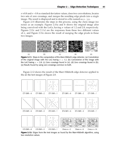
Figure 2.12 shows the result of the Marr-Hildreth edge detector applied to
the all the test images of Figure 2.8.

ET1 SNR = 6 ET1 SNR = 2 ET1 SNR = 1 ET1 SNR = 6 ET1 SNR = 2 ET1 SNR = 1

ET3 SNR = 6 ET3 SNR = 2 ET3 SNR = 1 ET4 SNR = 6 ET4 SNR = 2 ET4 SNR = 1

ET5 SNR = 6 ET5 SNR = 2 ET5 SNR = 1 Chess σ = 3 Chess σ = 9 Chess σ = 18
Figure 2.12: Edges from the test images as found by the Marr-Hildreth algorithm, using
two resolution values.