Page 182 -

162 CHAPTER 4 LINEAR PROGRAMMING APPLICATIONS

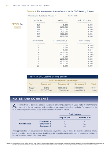
Figure 4.5 The Management Scientist Solution for the DOC Blending Problem

Objective Function Value = 9300.000

Variable Value Reduced Costs
-------------- --------------- -----------------
EXCEL file X1R 0.000 0.000
X2R 8000.000 0.000
DOC
X3R 2000.000 0.000
X1P 5000.000 0.000
X2P 2000.000 0.000
X3P 8000.000 0.000
Constraint Slack/Surplus Dual Prices
-------------- --------------- -----------------
1 0.000 0.580
2 0.000 0.480
3 0.000 0.240
4 3000.000 0.000
5 4000.000 0.000
6 0.000 0.000
7 1250.000 0.000
8 4000.000 0.000
9 3500.000 0.000
10 0.000 –0.080

Table 4.11 DOC Gasoline Blending Solution

litres of Component (percentage)
Fuel Component 1 Component 2 Component 3 Total
Regular 0 (0%) 8 000 (80%) 2 000 (20%) 10 000
1
1
1
Premium 5 000 (33 / 3 %) 2 000 (13 / 3 %) 8 000 (53 / 3 %) 15 000
NOTES AND COMMENTS

convenient way to define the decision variables in a blending problem is to use a matrix in which the rows
A correspond to the raw materials and the columns correspond to the final products. For example, in the
DOC blending problem, we could define the decision variables as follows:

Final Products
Regular Fuel Premium Fuel

Component 1 x 1r x 1p
Raw Materials Component 2 x 2r x 2p
Component 3 x 3r x 3p

This approach has two advantages: (1) it provides a systematic way to define the decision variables for any
blending problem; and (2) it provides a visual image of the decision variables in terms of how they are related to
the raw materials, products and each other.

Copyright 2014 Cengage Learning. All Rights Reserved. May not be copied, scanned, or duplicated, in whole or in part. Due to electronic rights, some third party content may be suppressed from the eBook and/or eChapter(s). Editorial review has
deemed that any suppressed content does not materially affect the overall learning experience. Cengage Learning reserves the right to remove additional content at any time if subsequent rights restrictions require it.