Page 319 -

TRANSPORTATION SIMPLEX METHOD: A SPECIAL-PURPOSE SOLUTION PROCEDURE 299

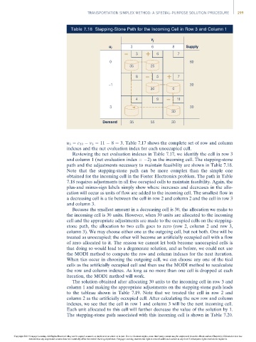
Table 7.18 Stepping-Stone Path for the Incoming Cell in Row 3 and Column 1
v j

u i 3 6 8 Supply
– 3 + 6 7
0 60
35 25

8 – 5 + 7

–1 30
30 0
4 9 – 11

3 30
30

Demand 35 55 30

u 3 ¼ c 33 v 3 ¼ 11 8 ¼ 3. Table 7.17 shows the complete set of row and column
indexes and the net evaluation index for each unoccupied cell.
Reviewing the net evaluation indexes in Table 7.17, we identify the cell in row 3
and column 1 (net evaluation index ¼ 2) as the incoming cell. The stepping-stone
path and the adjustments necessary to maintain feasibility are shown in Table 7.18.
Note that the stepping-stone path can be more complex than the simple one
obtained for the incoming cell in the Foster Electronics problem. The path in Table
7.18 requires adjustments in all five occupied cells to maintain feasibility. Again, the
plus-and minus-sign labels simply show where increases and decreases in the allo-
cation will occur as units of flow are added to the incoming cell. The smallest flow in
a decreasing cell is a tie between the cell in row 2 and column 2 and the cell in row 3
and column 3.
Because the smallest amount in a decreasing cell is 30, the allocation we make to
the incoming cell is 30 units. However, when 30 units are allocated to the incoming
cell and the appropriate adjustments are made to the occupied cells on the stepping-
stone path, the allocation to two cells goes to zero (row 2, column 2 and row 3,
column 3). We may choose either one as the outgoing cell, but not both. One will be
treated as unoccupied; the other will become an artificially occupied cell with a flow
of zero allocated to it. The reason we cannot let both become unoccupied cells is
that doing so would lead to a degenerate solution, and as before, we could not use
the MODI method to compute the row and column indexes for the next iteration.
When ties occur in choosing the outgoing cell, we can choose any one of the tied
cells as the artificially occupied cell and then use the MODI method to recalculate
the row and column indexes. As long as no more than one cell is dropped at each
iteration, the MODI method will work.
The solution obtained after allocating 30 units to the incoming cell in row 3 and
column 1 and making the appropriate adjustments on the stepping-stone path leads
to the tableau shown in Table 7.19. Note that we treated the cell in row 2 and
column 2 as the artificially occupied cell. After calculating the new row and column
indexes, we see that the cell in row 1 and column 3 will be the next incoming cell.
Each unit allocated to this cell will further decrease the value of the solution by 1.
The stepping-stone path associated with this incoming cell is shown in Table 7.20.

Copyright 2014 Cengage Learning. All Rights Reserved. May not be copied, scanned, or duplicated, in whole or in part. Due to electronic rights, some third party content may be suppressed from the eBook and/or eChapter(s). Editorial review has
deemed that any suppressed content does not materially affect the overall learning experience. Cengage Learning reserves the right to remove additional content at any time if subsequent rights restrictions require it.