Page 316 -

296 CHAPTER 7 TRANSPORTATION, ASSIGNMENT AND TRANSSHIPMENT PROBLEMS

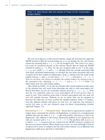
Table 7.13 New Solution After One Iteration in Phase II of the Transportation
Simplex Method

Boston Dubai Singapore London Supply
3 2 7 6
Czech 3 500 1 500
Republic 5 000

7 5 2 3
Brazil 2 500 2 000 1 500 6 000

2 5 4 5
China 2 500 2 500

Demand 6 000 4 000 2 000 1 500

We now try to improve on the current solution. Again, the first step is to apply the
MODI method to find the best incoming arc, so we recalculate the row and column
indexes by requiring that u i + v j ¼ c ij for all occupied cells. The values of u i and v j
can easily be calculated directly on the tableau. Recall that we begin the MODI
method by setting u 1 ¼ 0. Thus, for the two occupied cells in row 1 of the table,
v j ¼ c 1j ; as a result, v 1 ¼ 3 and v 2 ¼ 2. Moving down the column associated with
each newly calculated column index, we calculate the row index associated with each
occupied cell in that column by subtracting v j from c ij . Doing so for the newly found
column indexes, v 1 and v 2 , we find that u 3 ¼ 2 3 ¼ 1 and that u 2 ¼ 5 2 ¼ 3.
Next, we use these row indexes to calculate the column indexes for occupied cells in
the associated rows, obtaining v 3 ¼ 2 3 ¼ 1 and v 4 ¼ 3 3 ¼ 0. Table 7.14
shows these new row and column indexes.
Also shown in Table 7.14 are the net changes (the circled numbers) in the value
of the solution that will result from allocating one unit to each unoccupied cell.
Recall that these are the net evaluation indexes given by e ij ¼ c ij u i v j .Note
that the net evaluation index for every unoccupied cell is now greater than or
equal to zero. This condition shows that if current unoccupied cells are used, the
cost will actually increase. Without an arc to which flow can be assigned to
decrease the total cost, we have reached the optimal solution. Table 7.15 summa-
rizes the optimal solution and shows its total cost. As expected, this solution is
exactly the same as the one obtained using the linear programming solution
approach (Figure 7.2).

Maintaining m + n 1 Occupied Cells Recall that m represents the number of
origins and n represents the number of destinations. A solution to a transportation
problem that has less than m + n 1 cells with positive allocations is said to be
degenerate. The solution to the Foster Electronics problem is not degenerate; six
cells are occupied and m + n 1 ¼ 3+4 1 ¼ 6. The problem with degeneracy
is that m + n 1 occupied cells are required by the MODI method to compute all
the row and column indexes. When degeneracy occurs, we must artificially create an
occupied cell in order to compute the row and column indexes. Let us illustrate how
degeneracy could occur and how to deal with it.

Copyright 2014 Cengage Learning. All Rights Reserved. May not be copied, scanned, or duplicated, in whole or in part. Due to electronic rights, some third party content may be suppressed from the eBook and/or eChapter(s). Editorial review has
deemed that any suppressed content does not materially affect the overall learning experience. Cengage Learning reserves the right to remove additional content at any time if subsequent rights restrictions require it.