Page 312 -

292 CHAPTER 7 TRANSPORTATION, ASSIGNMENT AND TRANSSHIPMENT PROBLEMS

identify an incoming arc. The incoming arc is the currently unused route (unoccu-
pied cell) where making a flow allocation will cause the largest per-unit reduction in
total cost. Flow is then assigned to the incoming arc, and the amounts being shipped
over all other arcs to which flow had previously been assigned (occupied cells) are
adjusted as necessary to maintain a feasible solution. In the process of adjusting the
flow assigned to the occupied cells, we identify and drop an outgoing arc from the
solution. So, at each iteration in phase II, we bring a currently unused arc (unoccu-
pied cell) into the solution, and remove an arc to which flow had previously been
assigned (occupied cell) from the solution.
To show how phase II of the transportation Simplex method works, we must
explain how to identify the incoming arc (cell), how to make the adjustments to the
other occupied cells when flow is allocated to the incoming arc and how to identify
the outgoing arc (cell). We first consider identifying the incoming arc.
As mentioned, the incoming arc is the one that will cause the largest reduction
per unit in the total cost of the current solution. To identify this arc, we must
compute for each unused arc the amount by which total cost will be reduced by
shipping one unit over that arc. The modified distribution or MODI method is a way
to make this computation.
The MODI method requires that we define an index u i for each row of the
tableau and an index v j for each column of the tableau. Calculating these row and
column indexes requires that the cost coefficient for each occupied cell equal u i + v j .
So, since c ij is the cost per unit from origin i to destination j, u i + v j ¼ c ij for each
occupied cell. Let us return to the initial feasible solution which we found using the
minimum cost method (see Table 7.9), and use the MODI method to identify the
incoming arc.
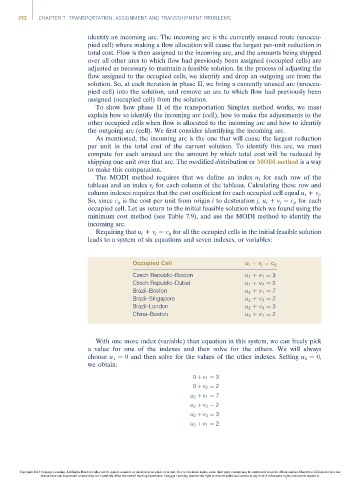
Requiring that u i + v j ¼ c ij for all the occupied cells in the initial feasible solution
leads to a system of six equations and seven indexes, or variables:

Occupied Cell u i + v j ¼ c ij

Czech Republic–Boston u 1 + v 1 ¼ 3
Czech Republic–Dubai u 1 + v 2 ¼ 2
Brazil–Boston u 2 + v 1 ¼ 7
Brazil–Singapore u 2 + v 3 ¼ 2
Brazil–London u 2 + v 4 ¼ 3
China–Boston u 3 + v 1 ¼ 2

With one more index (variable) than equation in this system, we can freely pick
a value for one of the indexes and then solve for the others. We will always
choose u 1 ¼ 0 and then solve for the values of the other indexes. Setting u 1 ¼ 0,
we obtain:
0 þ v 1 ¼ 3
0 þ v 2 ¼ 2
u 2 þ v 1 ¼ 7
u 2 þ v 3 ¼ 2
u 2 þ v 4 ¼ 3
u 3 þ v 1 ¼ 2

Copyright 2014 Cengage Learning. All Rights Reserved. May not be copied, scanned, or duplicated, in whole or in part. Due to electronic rights, some third party content may be suppressed from the eBook and/or eChapter(s). Editorial review has
deemed that any suppressed content does not materially affect the overall learning experience. Cengage Learning reserves the right to remove additional content at any time if subsequent rights restrictions require it.